A Buffer
In this post, we will discuss one of the most simple logic gates, a buffer.
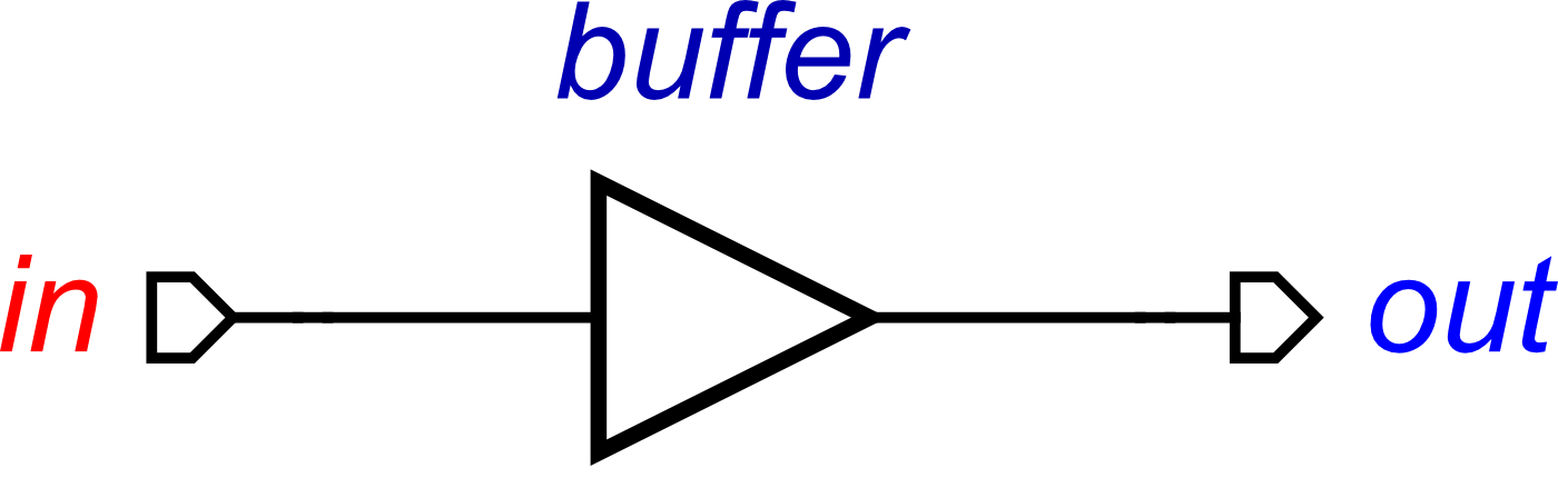
A buffer takes an input signal, and outputs a signal in the same state as the input signal, the output simply follows the input. For example, if the input signal changes from 0 to 1, the output will eventually change from 0 to 1. We say the output changes ‘eventually’ because the output changes after some unknown delay. It is possible for the input to change from 0 to 1, and then back to 0 very quickly, before we see any changes on the output. But intuitively, we want to be able to say that if the input transitions from 0 to 1, then stays 1 long enough, the output will follow and also transition to 1.
So how can we design these using concepts? We need to describe the causal relationship between the input and output; what occurs in the input to cause a transition in the output? For a buffer, this is when a signal transition occurs on the input, this needs to be reflected on the output. This can be described as:
buffer(in, out) = in+ ⇝ out+ ⋄ in- ⇝ out-
There are some operators to discuss here:
⇝ – Shows the causal relationship
⋄ – The composition operator
This concept therefore implies that in+ causes out+, this is composed with in- causing out-. This covers all the operations of the buffer.
But now, how does this turn into a Signal Transition Graph, which we can simulate, verify and test to ensure it works correctly? This is performed using an algorithm:
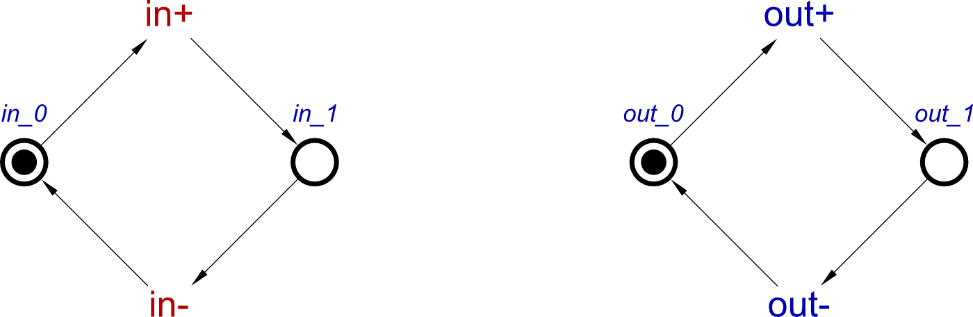
First of all, the algorithm takes the list of concepts and finds places one of these cycle for each individual signal. This is to keep with the property of consistency, where positive (+) and negative (–) transitions of each signal must always alternate. This is also in-keeping with the possibility for a signal to transition one way and back quickly without affecting the others, as with the example of the input transitioning high and then low before the output changes.
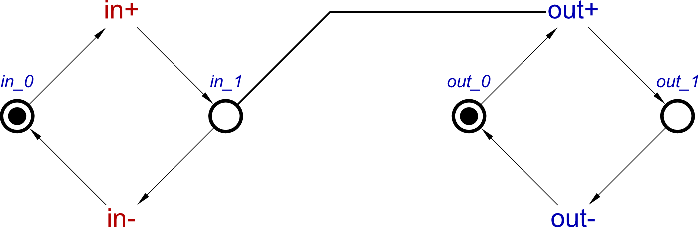
Next, the algorithm uses the first concept, in+ ⇝ out+, to show this causality in the STG. This concept shows how the input rising causes the output to rise, so this is viewed in an STG by connecting the in_1 place, which shows when the input has transitioned high, to the transition of out+. This is done using an arc commonly known as a read-arc. This is because a one way arc connecting these STG components would mean that when out+ occurs, a token in in_1 is consumed, blocking in- from being enabled. A read-arc allows out+ to simply check for a token in in_1 for it to occur without consuming it.
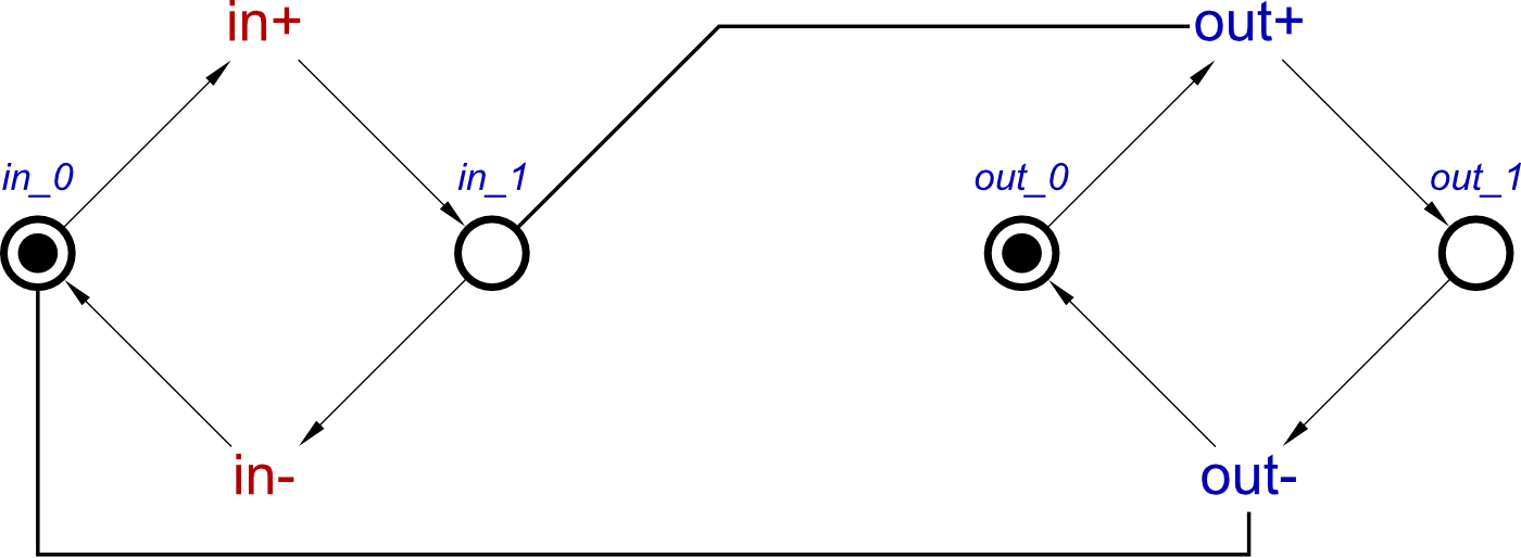
In the final step for designing a buffer, another read arc is used which represents the concept of in- ⇝ out-, connecting in_0 place with the out- transition. This conversion of a concept to an STG is now complete.
Note that in the above STGs we assume that all signals are initialised to 0. In a later blog post we will see how to use concepts to specify initial states of all signals in a compositional manner.
Reuse
Now we have defined a buffer, we can reuse this. As said earlier in this post, a concept can be defined as several concepts. Therefore, let use an example of a circuit which uses buffers.
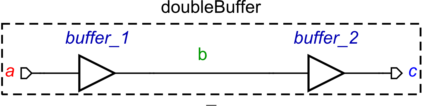
This circuit can be produced from the following concept:
doubleBuffer = buffer(a,b) ⋄ buffer(b,c)
In this circuit, a is an input, c is an output, and b is an internal signal connecting the output of buffer_1 to the input of buffer_2. We could have described this using signal-level concepts, which would be a longer description that that of the one above. Since we have defined a buffer, we can simply reuse this definition in order to save time on describing concepts. This produces the following Signal Transition Graph:
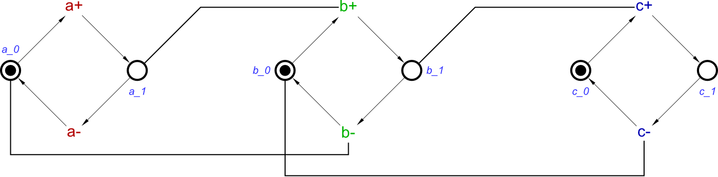
Comparing this STG to the STG for a single buffer, it is possible to see that a and b in this STG form one buffer, and b and c form another buffer. Again, we assume that all signals are initially 0.
Finally
In this first blog post, we have discussed how to describe a simple logic gate, a buffer, in terms of concepts. How these concepts are then converted into a Signal Transition Graph is also described. Another useful aspect of concepts is their reusability, and how a defined concept can be reused is displayed in an example using two buffers.
The following post, Concepts II: An inverter will discuss another simple logic gate, an inverter. After having defined these two gates, a further post will explain how initial states work, whether defined as part of a concept or not, using both a buffer and an inverter as examples.