All posts by b0093796

Concepts VI: OR-causality – Part 2

As discussed in Part 1, OR-causality is a useful and important part of specifying circuits, and with our recently released tool (https://github.com/tuura/concepts), we needed to include OR-causality in the translation from concepts to STGs.

To include this in the tool, we needed to design an algorithm which can take OR-causality, and seamlessly use it in conjunction with standard AND-causality.

This part will detail our algorithm. Our tool is written in Haskell, and while some of the algorithm is based on Haskell constructs, we will aim to use pseudo code to describe this algorithm.

OR-causality, an algorithm

For an example to explain this, we will use Example 2 from Part 1 of this post, an OR-Gate with a single AND-causality. This will display well OR- and AND-causality interaction.

Let’s just remind ourselves of the concepts for this:

circuit  = orGate a b c ⋄ buffer d c

This can also be described using signal-level concepts:

circuit = [a+, b+] ~|~> c+ ⋄ a- ⇝ c- ⋄ b- ⇝ c- ⋄ d+ ⇝ c+ ⋄ d- ⇝ c-

The first thing we need to think about is how we store this information. As we said in Part 1, OR-causality is described by listing the possible causes for a single effect, for example from:

[a+, b+] ~|~> c+

We can see that a+ and b+ are the possible causes for the c+ effect transition.

Therefore, we can list OR-causality as a list of causes for each effect. However, this will cause issues when there is more than one list of OR-causality causes for a single effect, but we will discuss this later.

This also causes an issue with AND-causality causes, as we cannot simply add these to the list of OR-causality causes, as this would change the type of causality from AND to OR.

To solve this problem, we treat each type of causality as a separate list, where OR-causality is a list of at least two causes, and AND-causality is a list with a single cause. These are stored with the corresponding effect to the causality. So, for c+ in this example, we would store:

Causes: [a+, b+] & Effect: c+
Causes: [d+] & Effect: c+

Now, looking back at the example, the resulting STG features two c+ transitions, but how do we arrive at the number of transitions we need?

The next step in this algorithm is to rearrange these stored lists of effects so we then have the cause transitions required for each of the resulting effect transitions, c+ in this case, to be able to occur. This is done using the Cartesian Product, commonly used in mathematics to “expand the brackets”, which, due to how lists are stored, also applies here. The Cartesian product will produce a number of results, based on the size of the inputs. In this case, we have two lists, one of size 2 and one of size 1. Multiplying these numbers gives us 2 results, and thus, 2 effect transitions.

With that in mind, we need to perform the Cartesian product on these two lists, which will provide us with two new lists which are the effects required per cause transition. This will be performed as follows:

1 – [a+, b+] * [d+] — The original lists
2 – [a+ * d+], [b+ * d+] — A list of lists after performing the Cartesian product on 1

2 holds a list of lists, each list being the required effects for a single transition to occur, one requiring both a+ and d+, the other requiring both b+ and d+. Due d+ being in an AND-causality relationship with c+, it is required to have occurred, regardless of whether a+ or b+ has occurred.

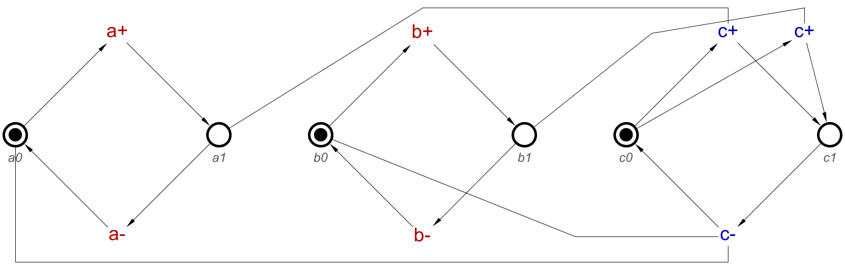
Now we need to include the two c+ transitions in the output of the tool, to be included when importing into Workcraft. The tool outputs the STG in dotG format, which is commonly used by existing tools which work with STGs. This format allows for the inclusion of more than of the same signal transition. The first of each transition will be output as expected, c+, but a second one will be output as c+/1. A third will be known as c+/2, and so on. For this example we will have c+ and c+/1.

With this information, we can now apply the specific transitions to the lists we have for each transition:

Causes: [a+, d+] & Effect: [c+]
Causes: [b+, d+] & Effect: [c+/1]

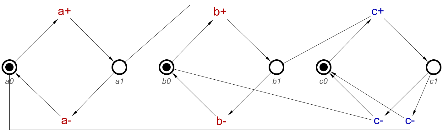
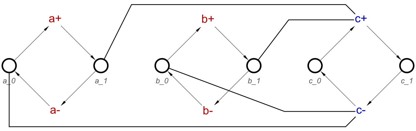
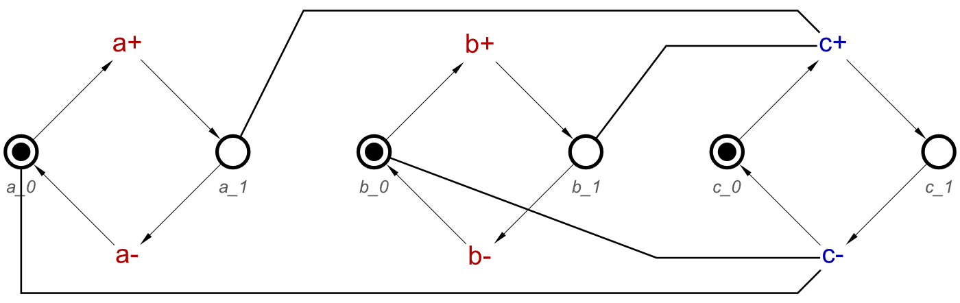
And this can now be converted to the transitions and read-arcs as expected, to produce the STG shown in Example 2 in Part 1 of this blog post.

A full example – 2 OR gates

Now we have discussed OR-causality, and the algorithm for this, let’s do an example from start to end, 2 OR gates. In this example, signals a, b, d and e are inputs, c will be the only output.

The concept for this is:

circuit = orGate a b c <> orGate d e c

Expanded into signal-level concepts, this is:

circuit = [a+, b+] ~|~> c+ ⋄ a- ⇝ c- ⋄ b- ⇝ c- ⋄
                    [d+, e+] ~|~> c+ ⋄ d- ⇝ c- ⋄ e- ⇝ c-

So, the tool will take these as these lists:

Causes: [a+, b+] & Effect: c+
Causes: [d+, e+] & Effect: c+

We now perform the Cartesian product on the two causes lists, which, knowing that there are two causes in each list, this will give us 4 c+ transitions. The result, with the transition names included will be:

Causes: [a+, d+] & Effect: [c+]
Causes: [a+, e+] & Effect: [c+/1]
Causes: [b+, d+] & Effect: [c+/2]
Causes: [b+, e+] & Effect: [c+/3]

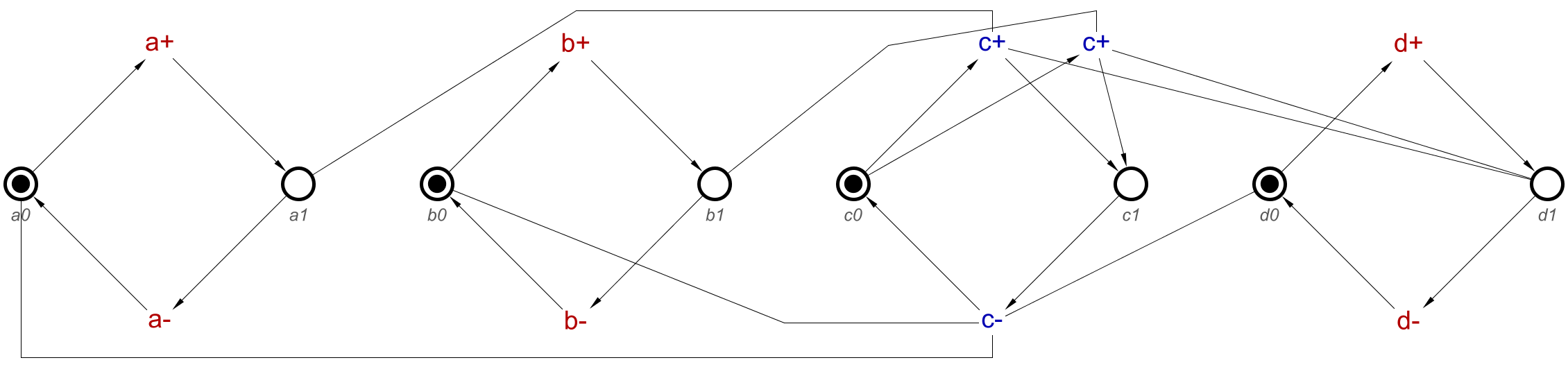
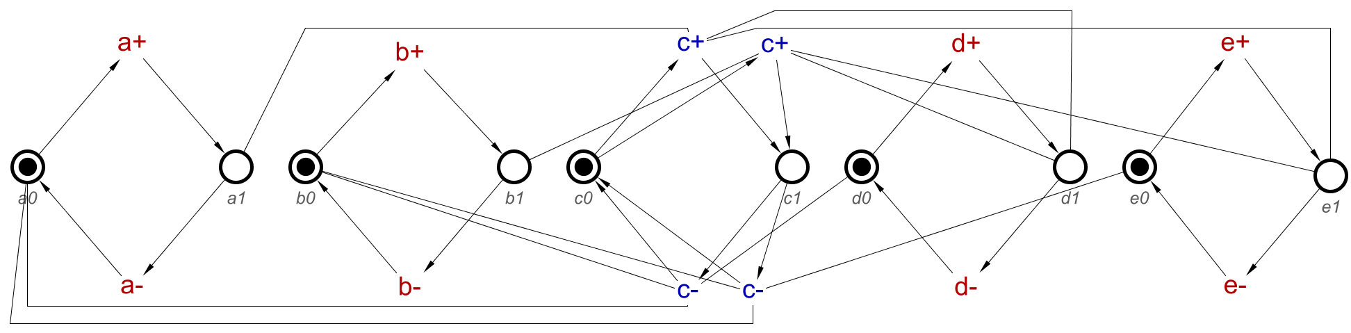
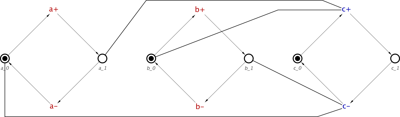
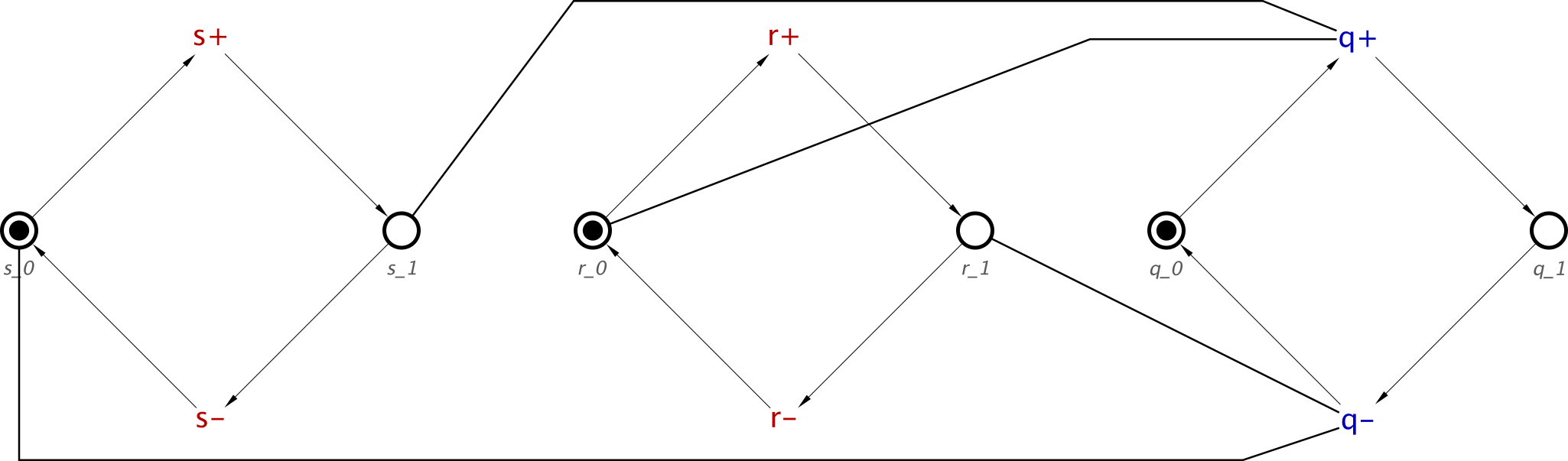
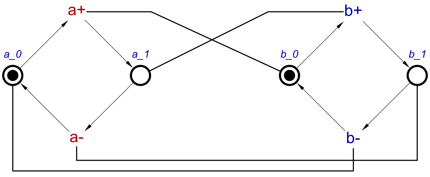
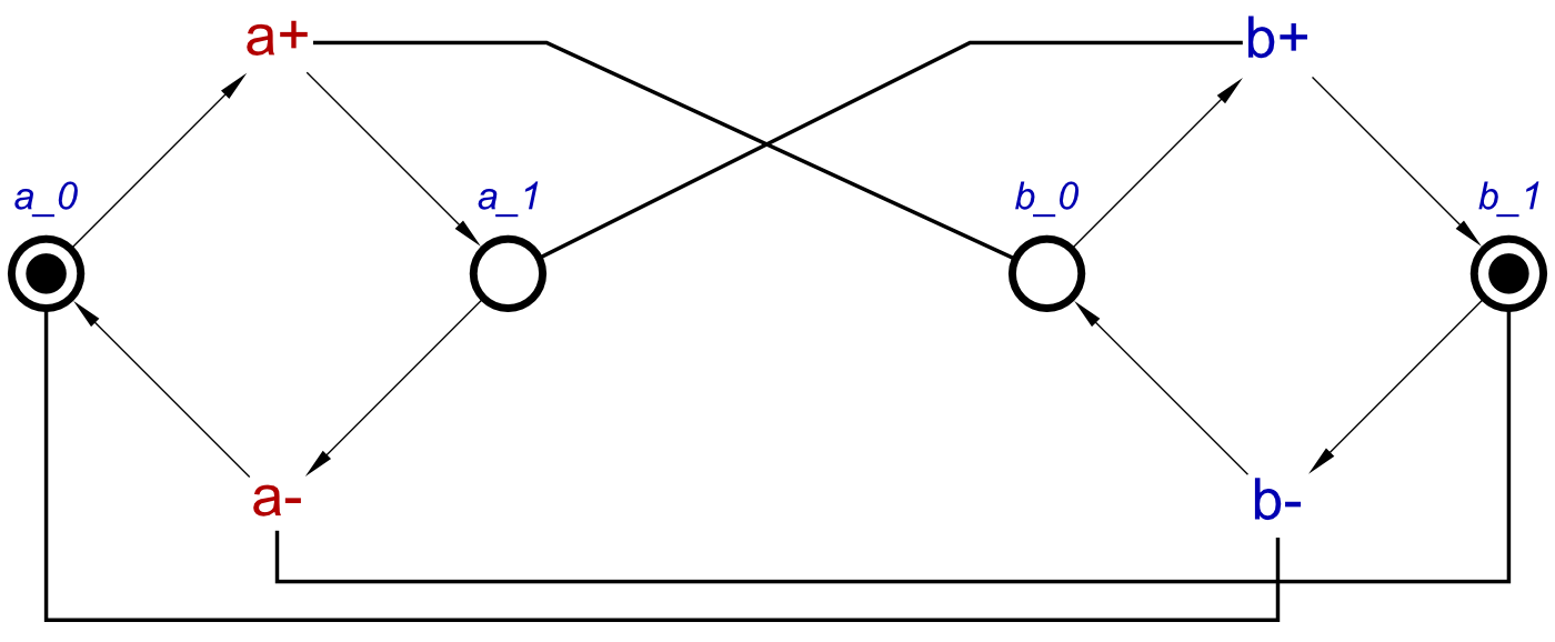
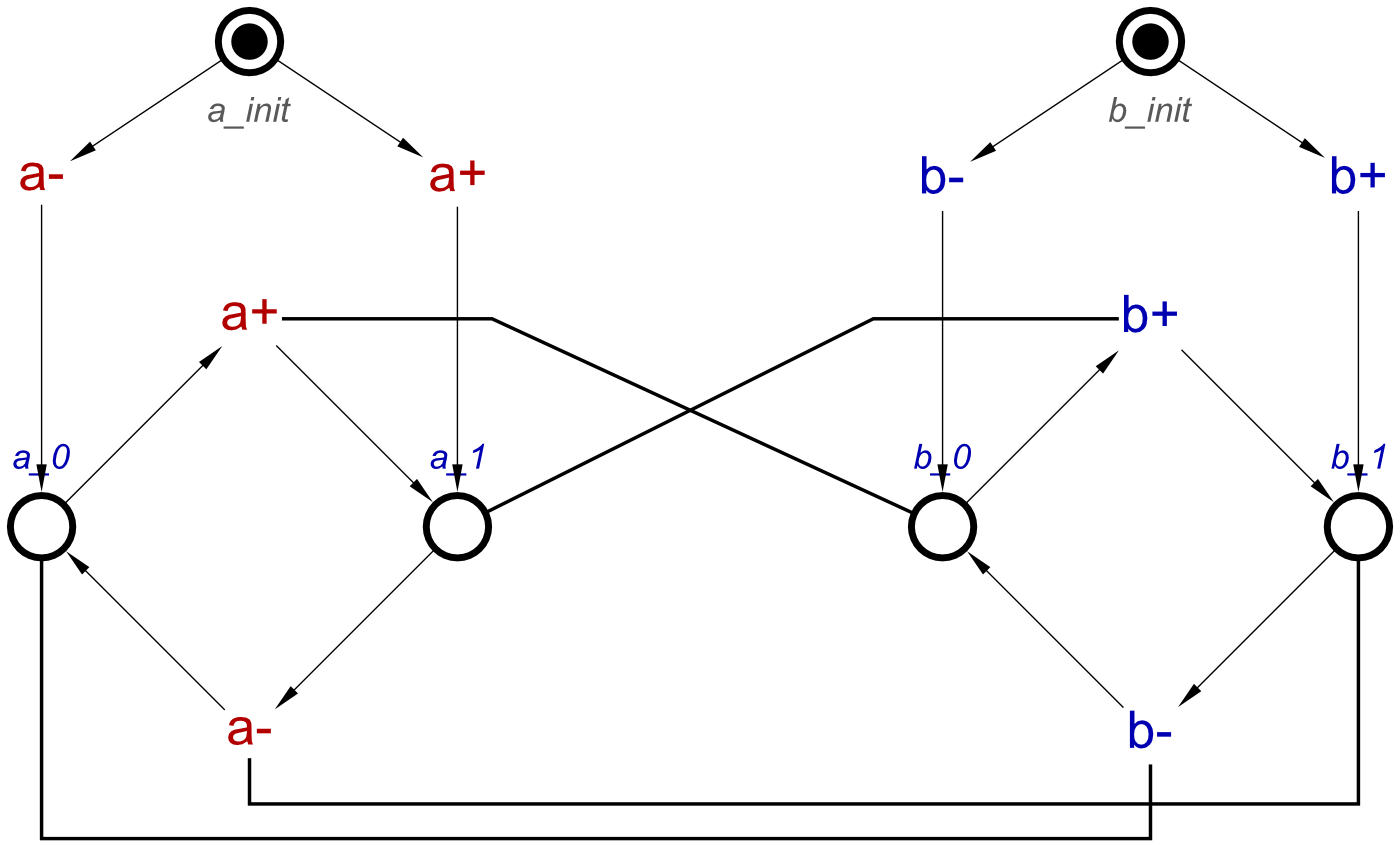
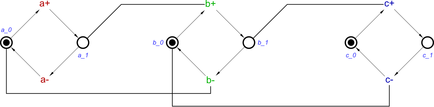
And this will translate to an STG like this:

2OrGates

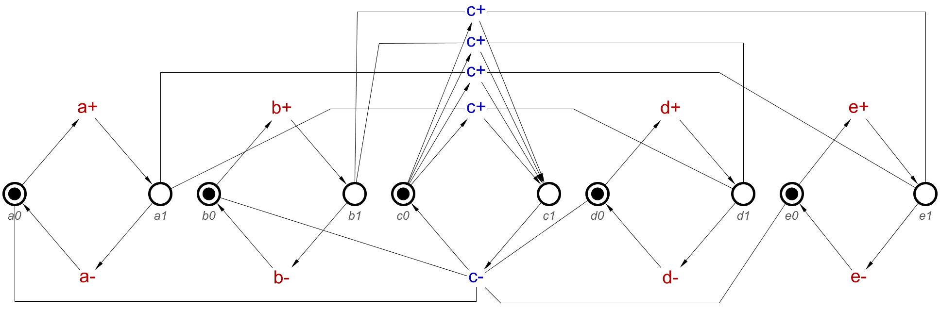
This clearly has 4 c+ transitions, and testing it proves that for any of them to allow any c+ to occur needs at least one of a+ and b+, as well as, at least one of d+ and e+. 

Finally

In both of these parts of the blog post, I have introduced OR-causality, and the algorithm to translate this to STGs. Through several examples, it can be seen that the algorithm works to produce STGs which display OR-causality.

The now released concepts translation tool can be effectively used to specify circuits with many functions, and the inclusion of OR-causality makes this better still.

The future of this blog series will include some concepts used in the translation process to specify signal types and initial states, which in turn serve as somewhat of a tutorial for the tool.

The tool is now available from https://github.com/tuura/concepts, which includes a manual to help with installation. It is also integrated with the STG plugin of Workcraft, and is included with a download of the latest version of Workcraft.

Concepts VI: OR-causality – Part 1

OR-causality is an interesting part of specification of circuits, specifically when using Signal Transition Graphs (STGs). We have recently released a translation tool for Concepts (available from https://github.com/tuura/concepts), which will take a set of concepts, and produce an STG specification for this. This includes both standard AND-causality, and OR-causality. OR-causality poses a challenge, as with STGs, and in this post we aim to discuss this.

This will be a 2 part series, with several examples to help explain OR-causality in this post, part 1, and an algorithm in part 2 to translate OR-causality concepts to STGs.

OR-causality, an introduction

For this, let’s use four simple examples. Here, we will assume initial states for all signals as 0.

  1. OR-Gate

A standard gate used in many applications, an OR-gate, and the associated causality,  is important and a good example to use to display OR-causality.

In concepts, an OR-gate is defined as follows:

orGate a b c = [a+, b+] ~|~> c+ ⋄ a- ⇝ c- ⋄ b- ⇝ c-

There are some operators to discuss here:

[a+ , b+] – This is how signal transitions are listed.
~|~> – This shows an OR-Causalilty relationship

In words, this is a composition of three concepts. First, either a+ or b+ cause c+. Then, a- causes c-, and b- causes c-.

This will mean that, when a+,  b+ or both of these occur, c+ can occur. But, for c- to occur, a- and b- must have occurred.

OR_gate

This is the STG produced from translating the OR-gate concept. This looks like any other STG we have shown on this blog, however notice that there are two c+ transitions. This is how OR-causality is displayed in STGs. When a+ occurs, one of the c+ transitions can occur. When b+ occurs, the other c+ transition can occur. If both a+ and b+ have occurred, then either of the c+ transitions can occur. However, both a- and b- can occur, then and only then can c- occur.

Notice, that for the c+ transition, there is OR-causality with a+ or b+, but for the c- transition, there is AND-causality with a- and b-.

2. OR-Gate with a single AND-causality

This is an OR-gate with inputs a and b, and output c, with another input signal dd will form a buffer with c, including some AND-causality as well. This way we can show how AND- and OR-Causality interact. In concepts this is:

circuit  = orGate a b c ⋄ buffer d c

And, expanded into signal-level concepts, this is:

circuit = [a+, b+] ~|~> c+ ⋄ a- ⇝ c- ⋄ b- ⇝ c- ⋄ d+ ⇝ c+ ⋄ d- ⇝ c-

In words, for c+ to occur, d+ must occur, and either b+ or c+. For c- to occur, all of a-b- and d- must occur.

So, as a thought experiment, if a+ and b+ have occurred, no c+ transition can occur without d+ having occurred.

The STG after translating the above concept is:OR_gate_1_AND_causality

Notice that this looks similar to the previous image, but with an extra consistency loop for the signal d. However, notice that d1, the place showing when d+ has occured, is connected to both c+ transitions. And d0 is connected to c-. This will therefore mean that, regardless of which of a+ or b+ have occured, c+ cannot occur without d+ occuring.

3. AND-Gate

Another standard gate. In this case, when thinking of it in terms of causality, it is the opposite of the OR-gate. i.e. For the c+ transition, there is AND-causality with both the a+ and b+ transition. Yet, with the c- transition, there is OR-causality between the a- and b- transitions.

The concepts for this is:

andGate a b c  = a+ ⇝ c+ ⋄ b+ ⇝ c+ ⋄ [a-, b-] ~|~> c-

This can be described in words as in the previous paragraph.

Let’s translate this to an STG.AND-Gate

Notice that this time, there are two c- transitions, as this transition is the OR-causality in an AND-gate. Notice the similarities between this and the OR-gate STG, just a sort-of mirror image.

4. AND-Gate and OR-Gate

For this, signals a and are the inputs to an OR-gate, and signals d and e are the inputs to an AND-gate. The outputs for both of these gates are c. Synthesizing this would not simply produce an AND and OR gate, but for this example, it shows how the AND and OR causality can interact in and interesting way.

This in concepts is:

circuit = orGate a b c <> andGate d e c

If we expand this:

circut = [a+, b+] ~|~> c+ ⋄ a- ⇝ c- ⋄ b- ⇝ c- ⋄
                  d+ ⇝ c+ ⋄ e+ ⇝ c+ ⋄ [d-, e-] ⇝ c-

In words, this means that for c+ to occur, either a+ or b+and both d+ and c+ must have occured. For c- to occur, both a- and b-, and either d- or e- must have occured.

This is slightly more confusing than the previous examples, and the resulting STG produced by translating this concept is interesting:

AND-OR-Gate

It does look a little confusing, but notice there are two of both c+ and c- transitions. Their interactions with the other signals determine which of these are able to transition. Testing this would prove that the concept description above works.

Finally

There is little reuse here. The concepts above feature some reuse of previously discussed concepts, but due to the inclusion of OR-causality, we cannot use any previously included gate- or protocol-concept as they do not feature any OR-causality.

So in this post, we have discussed OR-causality, and some uses of it. Specifically, I have aimed to show how it works on it’s own, and in conjunction with AND-causality.

Part 2 of this post will include an algorithm, as we have previously discussed how concepts are translated to STGs, but this algorithm will explain how OR-causality is translated, as this is quite specific.

Concepts V: Set-Reset Latch

Set-Reset Latch

After learning how a C-element can be produce with concepts, we can introduce other gates. In this case another fairly standard gate, a latch.

The operation of a latch is to hold a given value. There are several different types of latch, but in this case we will talk about a Set-Reset latch (SR Latch). This latch has two inputs, one will set the latch when high, causing its one output to be high. The second input will reset the latch when it is high, causing its output to be low.

So lets see how we can specify this using concepts.

Concepts

For this, let’s start off by referring to the two inputs as and b. The output is c.

So, first of all, lets think about how we can set the latch:

set = a+ ⇝ c+ ⋄ a- ⇝ c-

And it’s that simple. Simply put, when one of the outputs, a in this case, goes high, we want the output, c, to go high.

So we have described the interaction for set using one of the inputs and the output, now lets describe the reset action:

reset = b+ ⇝ c- ⋄ b- ⇝ c+

This will cause the output to go low when the second input, b, goes high.

These two concepts describe the operation of a SR-latch. But we still need to think about how the SR-latch will act initially, such as when it first receives power.

Unless specifically required, we should assume that the output of the latch should be low at startup. Because of this, we don’t want it to be set initially by a being high, so we can set this to 0 initially also.

However, with the second input, b, setting this high at this point would ensure that the output will reset to 0 at start up, but if the initial state of c is already set to low initially, we shouldn’t need to set to high, so we will set the initial state of this to low too.

The initial state concept will be as follows:

initialState = initialise(a, 0) ⋄ initialise(b, 0) ⋄ initialise(c, 0)

Now let’s create the scenario concept for the SR-Latch:

SRLatch = set ⋄ reset ⋄ initialState

And this can be converted to a Signal Transition Graph, so this specification can be verified, simulated, tested and then synthesised. The STG for a SRLatch will be as follows:

STG_SR_Latch

This is a fairly simple STG, but simulation would prove that setting high will allow c to transition high. Once it has transitioned high, it cannot transition low until b has been set high.

For some simpler understanding of how this latch works, we can change some of the signal names. In this case, we will change a to s, which stands for setwill be set to r, which stands for reset. Finally, we can call cq. q is a standard output symbol for latches.

This will change the concepts to the following:

set = s+ ⇝ q+ ⋄ s- ⇝ q-
reset = r+ ⇝ q- ⋄ r- ⇝ q+
initialState = initialise(s, 0) ⋄ initialise(r, 0) ⋄ initialise(q, 0)
SRLatch = set ⋄ reset ⋄ initialState

This will produce the following STG:STG_SR_Lath2

Changing the names of the signals does not affect the operation.

Now the SR-Latch has been defined, if a user has signals which will be inputs to a latch, they can use the concept and pass their signals into this, in the order of s, r and q.  For example someone can use the concept:

SRLatch(x, y, z)

In this case, x will be the set signal, y is the reset and z will be the output.

Some reuse

As is usually the case with concepts, we can define a SR-Latch using previously defined gates as concepts.

First of all, if we look at the set concept, it is clear that and form a buffer. So this can be rewritten as:

set = buffer(s, q)

The reset concept can also be redefined. In this case, it acts as an inverter:

reset = inverter(r, q)

As the initial state doesn’t need to be changed, we can compose these concepts as above to produce the SRLatch concept:

SRLatch = set ⋄ reset ⋄ initialState

Or we can reduce the number of concepts defined and compose these as follows:

SRLatch = buffer(s, q) ⋄ inverter(r, q) ⋄ initialState

There are of course several ways of specifying an SRLatch using concepts, but these are two of the simpler ways, either using signal-level concepts, or predefined gate-level concepts. The preference is entirely on the user.

Finally

In this post, we have explained another simple logic gate. The discussion includes the basic operation being specified as signal-level concepts, or by taking this a step higher and using pre-defined gates.

We have also shown how while the concept defines certain signal names, these aren’t set. A default SRLatch concept will use these signal names, but if these signals are not used in a design, a user can pass the desired signal names into the concept, and these names will replace the default ones.

This blog series will continue soon, with the inclusion of further logic gates and how they can be defined simply.

Concepts IV: C-Element

C-Element

Finally, after introducing the basics of concepts, we can now apply this to the design of logic gates. In this post, we will produce a very standard gate, a C-Element.

A C-Element’s basic operation is that, when all the inputs to the gate are high, or 1, then the output will be set high. This output will remain high until all of the inputs are low, or 0, at which point the output will be set low.

So let’s describe this using concepts!

Concepts

For this example, the C-Element we describe will be a 2 input gate. These will be and b.  The single output will be c. 

So let’s start with describing what causes the output to go high:

outputRise =  a+ ⇝ c+ ⋄ b+ ⇝ c+

This concept will cause the output, c, to go high when both the inputs, and b, are high.

Next, let’s describe what causes the output to go low:

outputFall =  a- ⇝ c- ⋄ b- ⇝ c-

Similar to the previous concept, outputFall will cause c to go low only when both and b are low.

And these two concepts describe the operation of a C-element. Let’s combine them, and then we can Convert them to an STG, giving us the following:

C-Element = outputRise ⋄ outputFall

C-Element1

In this state however, this STG is not particularly useful, as there are no initial states, and therefore it cannot be simulated or synthesized. Thus, let’s add an initial state concept:

initialState = initialise(a, 0) ⋄ initialise(b, 0) ⋄ initialise(c, 0)
CElement  = outputRise ⋄ outputFall ⋄ initialState

By setting all the initial states to 0, we can then test this STG using Workcraftand see that the STG (shown below) operates as a C-element.

C-Element2

This STG could also be tested by setting the initial states to any combination. The C-Element would still act as expected.

Some reuse

It is possible to describe a C-Element using predefined gates. If we break down some of the concepts used above we find some interesting points.

If we take the interactions of just one input signal and the output signal from the above concepts we get the following:

input1 = a+ ⇝ c+ ⋄ a- ⇝ c-

This concept is actually exactly the same as a gate we have previously defined: a buffer. Thus, a C-Element can actually be described using these:

CElement = buffer(a, b) ⋄ buffer(b, c) ⋄ initialState

The initial state must be included in order for the resulting STG to be usable in further operations.

Finally

This blog post has finally explained how concepts can be used to design a logic gate, albeit a simple one. This includes describing it’s operations in terms of the interactions of the input and output signals, or using predefined concepts, particularly a buffer.

The next post will continue in the effort to define logic gates using behavioural concepts, the next being an Set-Reset Latch

Concepts III: Initial States

Initial States

Now we have introduced a couple of simple gates, a buffer and an inverter, we should now discuss an important part of Signal Transition Graphs, and their implementation using Concepts. These are initial states.  

Initial states are used in Signal Transition Graphs to show what state a signal is in, high or low, when the system being designed starts. This is important as STGs require initial states for simulation, verification and synthesis.

In the previous posts, we have assumed that all signals involved in the STGs are initially set to 0, and this has been indicated by placing a token in the places which are before each signals transition (as above), but this assumption cannot be applied to every STG.

Example – A Handshake

So now let’s use a previous example, a Handshake, and discuss what we can do to ensure there are initial states in an STG produced using concepts.

The concept used to describe a handshake is as follows:

handshake(a,b) = buffer(a,b) ⋄ inverter(b,a)

This concept captures the interactions of signals a and b, using previously defined buffer and inverter concepts, but this does not explain the state of these signals when the handshake starts.

Initial state concepts can be defined similarly to other concepts, and thus can be composed with other concepts as normal. For this example, let’s say the two signals involved in handshake are both initially 0.

initialState = initialise(a,0) ⋄ initialise(b,0)

There is some syntax to discuss here:

initialise(a,0) – This is used to express an initial state. The state of the signal, a, will be initially set to 0.

The concept, initialState, implies that the initial state of signals and will be 0, so the first transition of each can be +, from low to high.

Now we can include this concept with the handshake concept:

system = handshake(a,b) ⋄ initialState

Passing this concept into the algorithm will produce the same STG as in the previous post:

bufferAndInverter00

And this can be resynthesized to produce the same handshake STG:

handshake00

However, what if the initial states are not both 0? For this, let’s redefine the initial state concept and compose this with a handshake concept:

initialState = initial(a,0) ⋄ initial(b,1)
system = handshake(a,b) ⋄ initialState

Now, a should initially be 0, and b should initialy be 1. The STG produced from these concepts is:

BufferAndInverter01This is the same as the previous version, but the tokens have shifted. After resynthesis, the STG is as follows:BufferAndInvertorRe01Again, very similar to the previous post-resynthesis STG. But in this case, we can see that b- is the first transition, instead of a+.

No initial state concepts

So, what if a set of concepts doesn’t contain any initial state concepts. In this case, the STG produced may still be a correct implementation of the system, but a user may wish to do some testing with options for initial states open.

When this occurs, the algorithm has the option of adding some extra transitions to allow a user some options. So, for example, let’s define a handshake, but no initial states:

system = handshake(a,b)

In this case, we make no assumptions of initial states, but how does this affect the STG produced?

BufferInverterNoInit

The STG produced is very similar to the previous STG, the concepts used to describe which features initial states. In this case however, the places a_0, a_1, b_0 and b_1 are all free from tokens. In order to select an initial state, the algorithm adds in an extra place and two extra transitions per signal, in order to allow  a choice of each signal’s initial state.

Using this example, when a user starts the simulation, the first transitions to be enabled will be the transitions either high or low from the initial state selections, allowing the user to select a- to set this signal to 0 initially, or a+ to set it to 1 initially, and this is the same as with signal b.

After this choice is made, the initial state selection will no longer be usable until the simulation is started again. The user can test how the system runs using these initial states, and then restart to test another combination of initial states. After the initial states have been selected, the user can either change this STG, removing the initial state selections and adding tokens into the correct place, or they can add the initial states to the list of concepts, and re-compose these for a new STG.

DISCLAIMER – An STG featuring initial state selection is not a correct STG, it violates properties of STGs which are necessary in order to be used with tools which perform useful functions like synthesis, for example. Currently, this method of testing for initial states should be used only for simulation, to test how differing initial states can affect a system. Any future developments are made on how to include a choice  of initial state in a correct STG, a follow-up post will be made.

Finally

In this and the previous two posts, we have covered the basics of concepts, and the design process of various simple gates.  Now we can move onto discussing some more complicated designs, and how we can use pre-existing concepts, and define new ones.

The next blog post will be Concepts IV: A C-element. This will be the first in a set of posts describing some standard logic gates, and from this we will work up to some more complex examples, using some of the previously described gates.

Concepts II: An inverter

An inverter

In the second post in the Concepts series we will discuss another simple logic gate, an inverter.

inverter

An inverter takes an input signal, and outputs a signal in the opposite, or inverted, state as the input signal, the output is simply the opposite of the input. For example, if the input signal changes from 0 to 1, the output will eventually change from 1 to 0. Similar to with the buffer, and the same with all gates, we say the output changes ‘eventually’ because the output changes after some unknown delay.

So how do we design an inverter using concepts? We need to describe what causes the output to transition, in terms of when the input transitions.  This can be described as:

inverter(in, out) = in+ ⇝ out- ⋄ in- ⇝ out+

This is very similar to the buffer concept, but with some subtle differences.  This concept implies that in+ causes out-.  This is composed with in- causing out+.  Therefore, this concept suggest that when the input transitions one way, the output will eventually transition in the opposite direction, for example, when in+ occurs, out- will eventually occur after, providing in stays high.

As with the previous post, we need to produce an STG from the inverter concept, which we can simulate, verify and test.  To do this, we pass this into the conversion algorithm, which starts as follows:

Buffer0

As with the buffer, it starts off by placing cycles for each individual signal.  This keeps the property of consistency in the STG, as discussed in Concepts I.

inverter1

Next, the first causality of the inverter concept is applied to these cycles.  This is in+ ⇝ out-. This connects the place after in+, labelled as in_1, with the signal transition of out-, using a read-arc. This is so that for out- to occur, in must have already transitioned high, which is displayed by in_1 possessing a token. The read-arc stops out- from consuming the token in in_1 which would block in- from happening, but allows out- to occur.

inverterSTG2

Finally, another read arc is used which represents the concept of in- out+, connecting in_0 place with the out+ transition. This conversion of a concept to an STG is now complete, and this correctly represents the operation of an inverter.

Note, as with the buffer STG, that in the above STGs we assume that all signals are initialised to 0.  In this case, it means that the output can initially transition high and will do eventually, due to the fact that in input is initially 0.

In a later blog post we will see how to use concepts to specify initial states of all signals in a compositional manner.

More reuse

We have now defined both an inverter and a buffer in these first two posts.  So lets use these together to show some reuse, and how these can be used together.

For this example, lets use a buffer and inverter loop.  It doesn’t necessarily have any real-world applications as these logic gates, but it’s a perfect example to show how concepts can be composed, and produces some interesting results.

bufferinverter

The signals shown in this diagram are simply used for viewing the outputs from the inverter and the buffer, but can be used as part of the concepts.

This circuit can be produced from the following concept:

bufferAndInverter = buffer(a,b) ⋄ inverter(b,a)

In this circuit, a is an input to the buffer, but the output from the inverter, and these are connected.  b is another signal connecting the output of the buffer to the input of the inverter.

As with the doubleBuffer example from the previous post, we could have described this using signal-level concepts, which would be a longer description that that of the one above. Since we have defined both an inverter and a buffer, we can simply reuse this definition in order to save time on describing concepts. The bufferAndInverter STG will be, assuming all signals are initially 0, as follows:

bufferAndInverterSTG

By following pairs of arcs, it is possible to see which are a cause of the buffer, and which are a cause of the inverter.  This STG can now be simulated, and does in fact act as expected from the circuit above.  When a+ occurs, b+ is enabled,  and after it transitions, this will cause a- to be enabled.  When a- has occurred, b- can then occur, after which a+ is enabled, and this completes the circuit.

This STG can be resynthesized, and the result is rather interesting:

handshake1

The resulting STG is in-fact the STG for a handshake protocol.  This means that what we have defined above, bufferAndInverter, is actually a handshake, described using a buffer and an inverter.  Therefore, let’s drop the current name, and re-define it using some parameters, so that any pair of signals can be handshaked.

handshake(a,b) = buffer(a,b) ⋄ inverter(b,a)

Handshakes are very useful for asynchronous systems, and having a concept defined for use at any time can make the design process much easier and quicker.

Finally

In this post, we have discussed how to describe a second logic gate, an inverter. We have described this in terms of concepts, and shown the conversion to produce an STG. We have also shown how a buffer and an inverter can be used in conjunction with one-another to produce a circuit, now that both have been pre-defined.

The next post, Concepts III: Initial States will use buffers and inverters as examples of how initial states can be defined using concepts, or in the case that initial states are not defined, how the conversion algorithm will apply options for initial states, so an STG produced can still be used for simulation.

Concepts I: A buffer

A Buffer

In this post, we will discuss one of the most simple logic gates, a buffer.

buffer_schematic

A buffer takes an input signal, and outputs a signal in the same state as the input signal, the output simply follows the input. For example, if the input signal changes from 0 to 1, the output will eventually change from 0 to 1. We say the output changes ‘eventually’ because the output changes after some unknown delay. It is possible for the input to change from 0 to 1, and then back to 0 very quickly, before we see any changes on the output. But intuitively, we want to be able to say that if the input transitions from 0 to 1, then stays 1 long enough, the output will follow and also transition to 1.

So how can we design these using concepts? We need to describe the causal relationship between the input and output; what occurs in the input to cause a transition in the output? For a buffer, this is when a signal transition occurs on the input, this needs to be reflected on the output.  This can be described as:

buffer(in, out) = in+ ⇝ out+ ⋄ in- ⇝ out-

There are some operators to discuss here:

⇝ – Shows the causal relationship
⋄  – The composition operator

This concept therefore implies that in+ causes out+, this is composed with in- causing out-.  This covers all the operations of the buffer.

But now, how does this turn into a Signal Transition Graph, which we can simulate, verify and test to ensure it works correctly? This is performed using an algorithm:

Buffer0

First of all, the algorithm takes the list of concepts and finds places one of these cycle for each individual signal. This is to keep with the property of consistency, where positive (+) and negative () transitions of each signal must always alternate. This is also in-keeping with the possibility for a signal to transition one way and back quickly without affecting the others, as with the example of the input transitioning high and then low before the output changes.

buffer1

Next, the algorithm uses the first concept, in+ out+, to show this causality in the STG. This concept shows how the input rising causes the output to rise, so this is viewed in an STG by connecting the in_1 place, which shows when the input has transitioned high, to the transition of out+. This is done using an arc commonly known as a read-arc. This is because a one way arc connecting these STG components would mean that when out+ occurs, a token in in_1 is consumed, blocking in- from being enabled. A read-arc allows out+ to simply check for a token in in_1 for it to occur without consuming it.

Buffer2

In the final step for designing a buffer, another read arc is used which represents the concept of in- out-, connecting in_0 place with the out- transition. This conversion of a concept to an STG is now complete.

Note that in the above STGs we assume that all signals are initialised to 0.  In a later blog post we will see how to use concepts to specify initial states of all signals in a compositional manner.

Reuse

Now we have defined a buffer, we can reuse this. As said earlier in this post, a concept can be defined as several concepts. Therefore, let use an example of a circuit which uses buffers.

double_buffer_schematic

This circuit can be produced from the following concept:

doubleBuffer = buffer(a,b) buffer(b,c)

In this circuit, a is an input, c is an output, and b is an internal signal connecting the output of buffer_1 to the input of buffer_2. We could have described this using signal-level concepts, which would be a longer description that that of the one above. Since we have defined a buffer, we can simply reuse this definition in order to save time on describing concepts. This produces the following Signal Transition Graph:

doubleBufferSTG

Comparing this STG to the STG for a single buffer, it is possible to see that a and b in this STG form one buffer, and b and c form another buffer.  Again, we assume that all signals are initially 0.

Finally

In this first blog post, we have discussed how to describe a simple logic gate, a buffer, in terms of concepts. How these concepts are then converted into a Signal Transition Graph is also described. Another useful aspect of concepts is their reusability, and how a defined concept can be reused is displayed in an example using two buffers.

The following post, Concepts II: An inverter will discuss another simple logic gate, an inverter. After having defined these two gates, a further post will explain how initial states work, whether defined as part of a concept or not, using both a buffer and an inverter as examples.

Designing asynchronous logic gates using behavioural concepts: An Introduction

Hello, and welcome to a series describing some of the more simple ideas of my PhD research, based on designing asynchronous circuits using concepts, an abstract language used to describe behaviours of specifications at signal, gate and protocol levels.

Simply put, concepts are a textual form of describing relationships between signal transitions in a system.  They are compositional and thus, several concepts can be composed to produce a new concept, which can then be composed with other concepts and so on.

Concepts can be used to describe smaller aspects of a system, such as causal relationships, initial states and quiescent transitions. However, due to their compositionality, they can be composed, and then used to describe logic gates or protocols and the transitions which occur within these. This removes the need to describe the signal interactions of gates and protocols, which can be lengthy, and a gate or protocol can simply be referred to by it’s name and the signals it uses.

This series will be used to discuss the design of logic gates using concepts.  Concepts are described using various operators which have been defined in a Haskell program, which serves as the backend for this method.  Any operators we meet in during this series will be described.

A graphical front end, Workcraft,will eventually be used for viewing Signal Transition Graphs (STGs) converted from concepts using an algorithm, which will be described in these posts.

The following posts in this series will begin by describing some simple gates, explaining how concepts are used to describe them. Then, how these are converted to produce an STG will be explained. Some other basic ideas of concepts and the conversion process will also be explained, for example, how initial states are applied, whether they are defined or not as concepts.

Following the basics, some more complex gates will be described, as well as how to make the descriptions of these gates simpler. This will all start with the following post: Concepts I: A buffer.