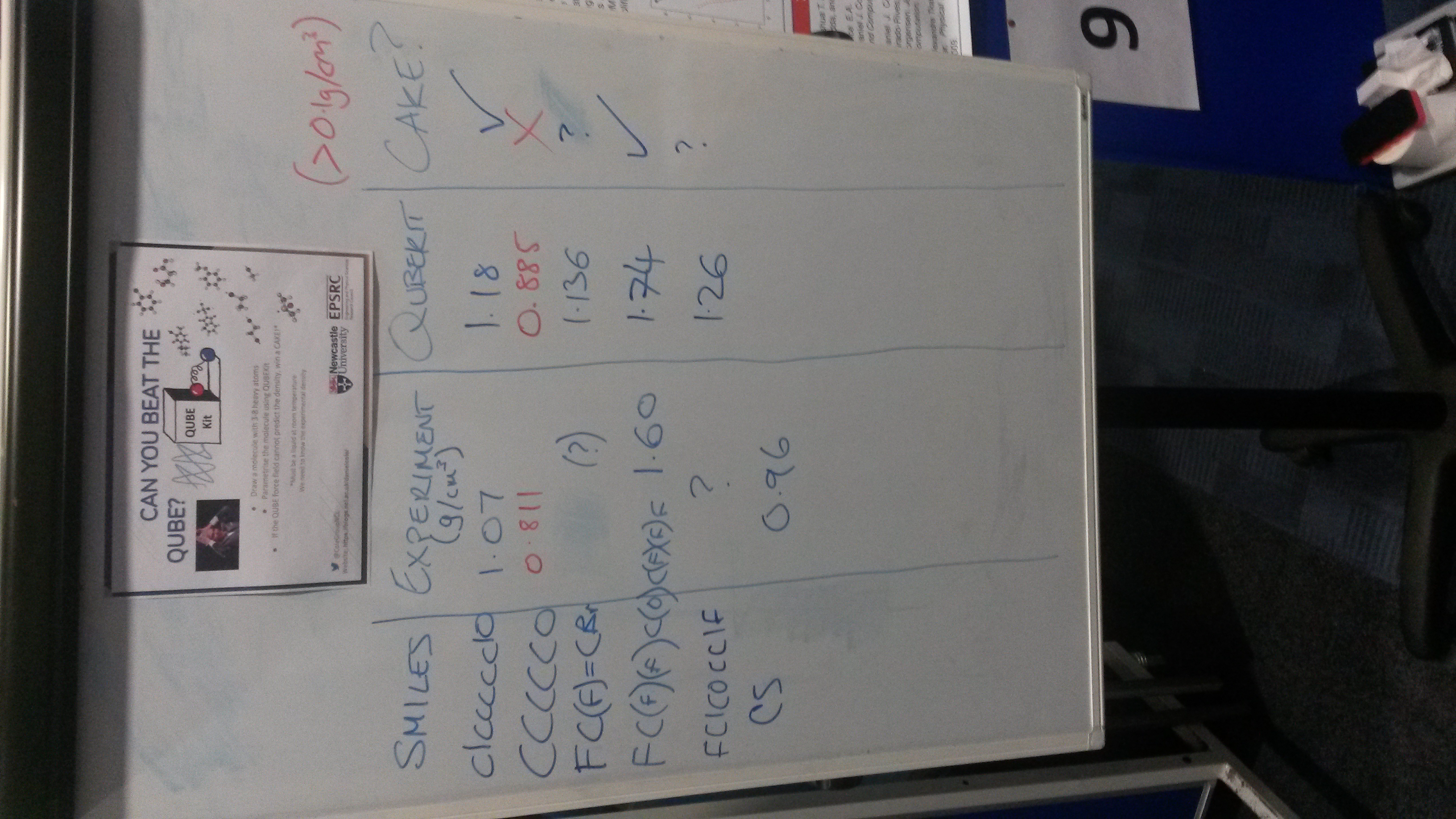
Can you beat the QUBE?
As part of the Newcastle SNES PGR conference we set out to demonstrate QUBEKit’s ability to quickly parametrise small organic molecules (between 3-8 heavy atoms) and then predict the liquid density – all in around 5 minutes.
Assuming you have QUBEKit and all of its dependencies set up, the following is a guide on how to recreate what we did.
Set-up
First we need to set up a config file for QUBEKit with the same execution settings, so by typing:
>>>QUBEKit -setup
A prompt will appear with options; select option 3 (make a normal config file)
>>>3
We created a demo.ini file by changing the quantum mechanical (QM) theory to B3LYP, the basis set to 6-31G*, the density engine was g09 (Gaussian 09) and DDEC6 was used to partition the electron density. We also gave each QM calculation 8 cores and 6 GB of memory (GPU: Quadro P5000, CPU: Intel Xeon(R) Gold 5118 CPU @ 2.30GHz). An example of the full ini file can be found in our github examples folder.
Execution
The participants were asked to draw a molecule of their choice on the LigParGen webserver. We then downloaded the PDB and XML files which are used as the inputs for QUBEKit.
The bond, angle, charge and Lennard-Jones parameters of each molecule were then derived directly from quantum mechanics; in the interest of time, torsions were not refit from their initial OPLS assigned values, and virtual sites were not used. Once the molecule was fully parameterised and the new OpenMM-ready XML files were produced, we were ready for a quick, pure liquid simulation.
Firstly, the insert-molecules function of GROMACS was used to create a box containing 267 replicas of the chosen molecule; this acts as our input for the pure-liquid simulation, along with the QUBEKit-generated XML file which contains the full force field. After googling the molecule’s experimental reference data and boiling point, an OpenMM simulation was started. A Jupyter notebook describing the simulation can be found here. In brief, the system is minimised, and then 20ps of molecular dynamics are used for equilibration, followed by a further 50ps for the production simulation. We then average the volume over the production run to get the density. The OPLS combination rules are used.
What happened?
Over the 2 hour session, seven molecules were parameterised (mostly limited by time spent talking to participants and searching for experimental data), three of which beat the simplified QUBEKit model since we could not predict the density to within 0.1 g/cm3 of the experimental value. For some of the constructed molecules, we could not find any experimental data to compare against, but we still demonstrated how easy the parametrisation process is with QUBEKit.
With more time, we can use higher level underlying quantum mechanical theory for parameterisation, and longer simulation times for the calculation of liquid density. For a more complete evaluation of QUBEKit accuracy, see here.
Next time, it would also be useful to see how participants cope interacting with QUBEKit by themselves. During the demonstration, we handled all of the simulations for them.
What’s the take home message?
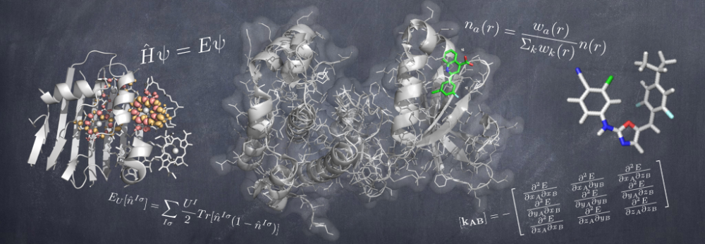
While liquid density might not be that interesting, it’s a useful measure of how well we’re treating interactions at the atomic scale. If we can predict liquid density to high accuracy, maybe soon we will be able to predict how strongly molecules bind to proteins and hence design new medicines.