Matt Grainger has kindly written this post about random encounter uncertainty models and camera traps
Random encounter models with camera traps
A recent paper in the Journal of Zoology by Tom Gray (“Monitoring tropical forest ungulates using camera-trap data” doi:10.1111/jzo.12547) used a random encounter model (REM) to assess the density of lesser oriental chevrotain Tragulus kanchil in the Southern Cardamom National Park, in south-west Cambodia. Random encounter models were adapted for camera trapping by Rowcliffe et al. (2008); these models allow estimates of populations of animals that are not individually-identifiable.
Density (D) is estimated from camera trap encounter rates by:
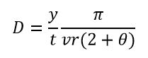
where y is the total number of photographs, t is the survey effort (camera-trap nights), v is the animals speed of movement and the camera detection zone is denoted by the radius (r) and angle (θ) of detection. The model assumes that camera traps are placed at random in relation to the animals movement. Variances can be estimated by non-parametric bootstrapping. Rowcliffe et al. (2008) suggest that the variances of the independently estimated variables (v, r and θ) can be incorporated by adding the squared coefficients of variation to that derived from bootstrapping to give an overall squared coefficient of variation for the density estimate.
Gray (2018) does not account for these variances in his paper, despite giving an indication of the size of the variation in these independently estimated variables. What difference would this make to the estimated density of lesser oriental chevrotain? Rather than using the delta method of Seber (1982) as suggested by Rowcliffe et al. (2008) I used the R package “propagate” (Spiess 2017) to propagate the uncertainty around the estimates of v, r and θ.
First we set up some data using the uncertainty estimates shown in Gray (2008).
set.seed(10101)
DAT <- data.frame(r = c(0.0014, 0.00026), v = c(0.82, 0.2),
                  y =c(501,0), theta =c(0.063,0),tm=c(8236,0),pi=c(pi,0))
Next we write the formula to estimate D as an expression.
EXPR <- expression((y/tm)*(pi/((v*r)*(2+theta))))
Then we can propagate the expression using the data. You can use the full data set or (as I have here) mean and standard deviations.
res <- propagate(EXPR, DAT)
We then convert the simulation results to a dataframe so we can plot it with ggplot2. Propagate has a plot function but I have not worked out how to customise it to my own liking yet.
dat <- as.data.frame(res$resSIM)
names(dat) <- "Density"
Let’s also look at the 95% highest density region (the credible interval) and the median density estimate from the simulation.
hdr(dat$Density, h = bw.nrd0(dat$Density))

 ## $hdr
 ##          [,1]     [,2]
 ## 99% -18.52657 213.3657
 ## 95%  19.59911 152.7857
 ## 50%  70.37278 109.9119
 ##
 ## $mode
 ## [1] 96.91486
 ##
 ## $falpha
 ##          1%          5%         50%
 ## 0.002749692 0.018249954 0.059715893

(median <- median(dat$Density))

## [1] 82.59773

lwr<-19.59#95% CI
uppr<-152.7857
Let’s plot the result of the simulation:
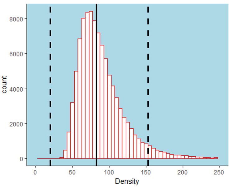
The simulated density of lesser oriental chevrotain when uncertainty is taken in to account (the median density value is indicated by the solid black line and the 95% credible interval is indicated by the dashed black lines).
In Gray (2018) density was estimated at 80.7 km-2 with boot-strapped 95% confidence intervals of 56.6-98.1 km-2. Here I have estimated density at 82.60 with 95% HDR 19.59 – 152.78 km-2. The median value is similar to the estimate in Gray (2018) but the credible intervals are much wider when we take uncertainty in to account. Given the wider credible intervals there is greater uncertainty in the estimate of density. Conservation managers might wish to increase the precision in the independently estimated variables by further research in to the species ecology (e.g. movement ecology) or by improving the estimate of the camera detection zone.
Decision making under uncertainty
With this approach we can ask questions related to the probability that the population density is greater than a value.
#What is the probability that the density is greater than 90 per Km-2?
sum(dat$Density>90)/dim(dat)[1]

## [1] 0.39562
These sorts of questions cannot easily be addressed outside of a Bayesian or simulation approach. This makes them extremely useful in decision making and wildlife monitoring. With monitoring data (e.g. several surveys over time) we can obtain the probability that the population is increasing or decreasing by a set amount.
References
Gray, T. (2018) Monitoring tropical forest ungulates using camera-trap data. Journal of Zoology, doi:10.1111/jzo.12547
Rowcliffe, J.M., Field, J., Turvey, S.T., Carbone, C. (2008) Estimating animal density using camera traps without the need for individual recognition. Journal of Applied Ecology, 45(4), 1228-1236
Seber, G.A.F. (1982). The estimation of animal abundance and related parameters. ISBN-13: 978-1930665552
Spiess, A-N. (2017). propagate: Propagation of Uncertainty. R package version 1.0-5. https://CRAN.R-project.org/package=propagate