Linking OpenLayers, D3, JSON and NetworkX to build a topological and geographic network viewer

As many of the networks that I am building as part of my involvement in the Infrastructure Transitions Research Consortium (ITRC – www.itrc.org.uk) are inherently spatial, I began thinking about how it might be useful to be able to visualise a network using the underlying geography but also as an alternative, the underlying topology. I began exploring various tools, and libraries and just started playing around with D3 (d3js.org).  D3 is a javascript library that offers a wealth of widgets and out-of-the-box visualisations for all sorts of purposes. The gallery for D3 can be found here. As part of these out-of-the-box visualisations it is possible to create force directed layouts for network visualisation. At this stage I began to think about I can get my network data, created by using some custom Python modules, nx_pg and nx_pgnet and subsequently stored within a custom database schema within PostGIS (see previous post here for more details), in a format that D3 can cope with. The easiest solution was to export a network to JSON format as the nx_pgnet Python modules allow a user to export a networkx network to JSON format (NOTE: the following tables labelled “ratp_integrated_rail_stations” and “ratp_integrated_rail_routes_split” were created as ESRI Shapefiles and then read in to PostGIS using the “PostGIS Shapefile and DBF Loader”).

Example Code:

import os

import osgeo.ogr as ogr

import sys

import networkx as nx

from libs.nx_pgnet import nx_pg

from libs.nx_pgnet import nx_pgnet

conn = ogr.Open(“PG: host=’localhost’ dbname=’ratp_networks’ user='<a_user>’ password='<a_password>'”)

 #name of rail station table for nodes and edges

int_rail_node_layer = ‘ratp_integrated_rail_stations’

int_rail_edge_layer = ‘ratp_integrated_rail_routes_split’

 #read data from tables and create networkx-compatible network (ratp_intergrated_rail_network)

ratp_integrated_rail_network = nx_pg.read_pg(conn, int_rail_edge_layer, nodetable=int_rail_node_layer, directed=False, geometry_precision=9)

 #return some information about the network

print nx.info(ratp_integrated_rail_network)

 #write the network to network schema in PostGIS database

nx_pgnet.write(conn).pgnet(ratp_integrated_rail_network, ‘RATP_RAIL’, 4326, overwrite=True, directed=False, multigraph=False)

 #export network to json

nx_pgnet.export_graph(conn).export_to_json(ratp_integrated_rail_network, ‘<folder_path>’, ‘ratp_network’)

 

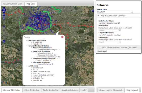
Having exported the network to JSON format (original data sourced from http://data.ratp.fr/fr/les-donnees.html), this was then used as a basic example to begin to develop an interface using D3 to visualise the topological aspects, and OpenLayers to visualise the spatial aspects of the network. A simple starting point was to create a basic javascript file that contained lists of networks that can be selected within the interface and subsequently viewed. Not only did this include a link to the underlying file that contained the network data, but also references to styles that can be applied to the topological or geographic views of the networks. A series of separate styles using the underlying style regimes of D3 and OpenLayers were developed such that a style selectable in the topological view used exactly the same values for colours, stroke widths, fill colours as styles applicable in the geographic view.  These stylesheets, stored within separate javascript files are pulled in via an AJAX call using jQuery to the webpage, subsequently allowing a user to select them. Any numeric attributes or values attached at the node or edge level of each network could also subsequently be used as parameters to visualise the nodes or edges in the networks in either view e.g. change edge thickness, or node size, for example. Furthermore, any attribute at the node or edge level could be used for label values, and these various options are presented via a set of simple drop down menu controls on the right hand side of the screen. As you may expect, when a user is interested in the topological view, then only the topological style and label controls are displayed, and vice versa for the geographic view.

For spatial networks, the geographic aspects of the data are read from a “WKT” attribute attached to each node and edge, via a WKT format reader to create vector features within an OpenLayers Vector Layer. It is likely this will be extended such that networks can be loaded directly from those being served via WMS, such as through Geoserver, rather than loading many vector features on the client. However for the purposes of exploring this idea, all nodes and edges within the interface on the geographic view can be considered as vector features. The NodeID, Node_F_ID, and Node_T_ID values attached to each node, or edge respectively as a result of storing the data within the custom database schema, are used to define the network data within D3.

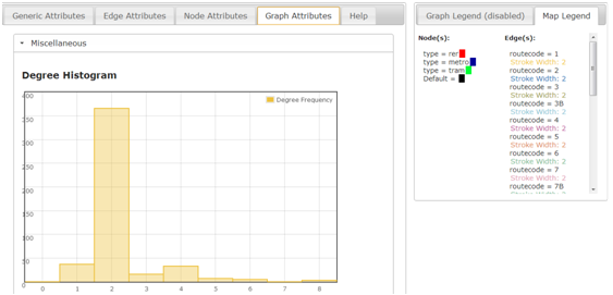
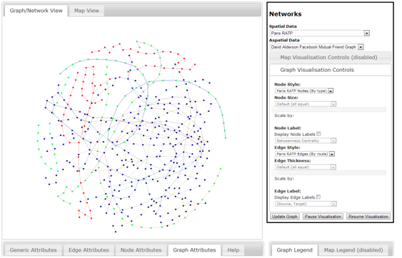
At this stage it is possible to view the topological or geographic aspects of the network within a single browser pane. Furthermore, if graph metrics have been calculated against a particular network and are attached at either the whole graph, or individual node or edge level, they too can be viewed within the interface via a series of tabs found towards the bottom. The following image represents an example of visualising the afore-mentioned Paris Rail network using the interface, where we can see that the controls mentioned, and how the same styles for the topological and geographic views are making it easier to understand where one node or edge resides within the two views. The next stage is to develop fully-linked views of a network such that selections made in one window are maintained within another. This type of tool can be particularly useful for finding disconnected edges via the topological view, and then finding out where that disconnected edge may exist in it’s true spatial location.