Computing connected components in an undirected graph is one of the most basic graph problems. Given a graph with n vertices and m edges, you can find its components in linear time O(n + m) using depth-first or breadth-first search. But what if you need to go faster? In this blog post, I will describe a cool new concurrent algorithm for this problem, which I learned this week at the Heidelberg Laureate Forum from Robert Tarjan himself. The algorithm distributes the work among n + m tiny processors that work concurrently most of the time and requires O(log n) global synchronisation rounds. The algorithm is remarkably simple but it’s far from obvious that it works correctly and efficiently. Happily, Tarjan and his co-author S. Cliff Liu have done all the hard proofs in their recent paper, so we can simply take the algorithm and use it.

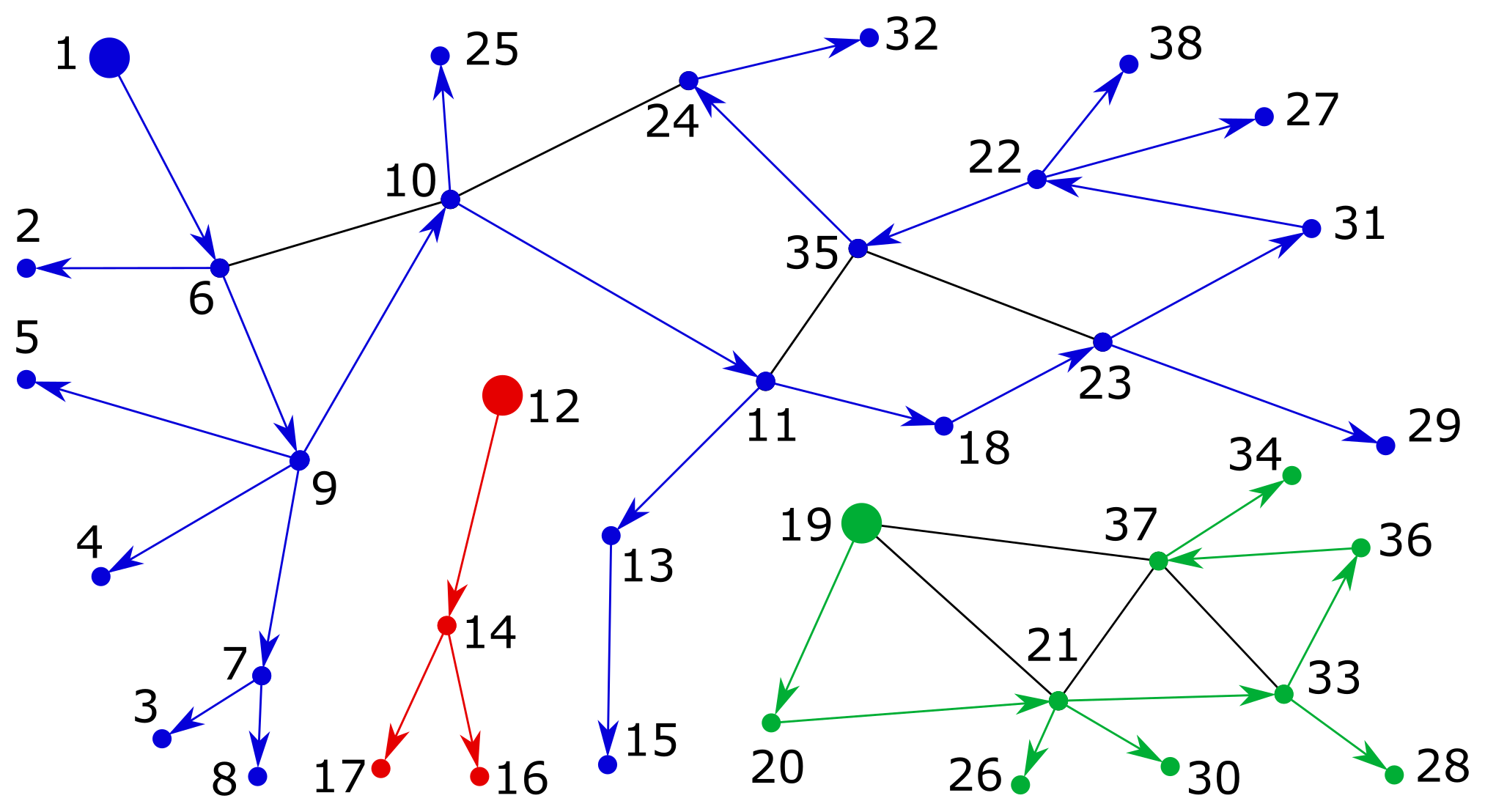
First, let’s recap the classic solution based on the depth-first search. I’ll use my favourite graph library Alga, so my examples will be in Haskell. Below I create an example undirected graph and compute the number of connected components by counting trees in the depth-first search forest. The graph and the forest are shown in the figure; the edges that belong to the forest are directed to illustrate the order of graph traversal.

λ> import Algebra.Graph.Undirected
λ> example = edges [ (1,6), (2,6), (3,7), ... ]
λ> length $ dfsForest $ fromUndirected example
3

This approach is very simple and you should definitely use it, provided that the linear complexity O(n + m) is fast enough for your application. But what if you need to go faster? Some time ago my colleagues and I wrote a paper where we showed how to take advantage of concurrency by implementing the breadth-first search on an FPGA, resulting in better time complexity O(d) where d is the diameter of the graph. This was an excellent result for our application where graphs had a small diameter, but in general, the diameter can be as large as n. So can we do better?

Yes! Tarjan’s paper presents several faster algorithms. It also describes the algorithms in a very nice compositional manner:

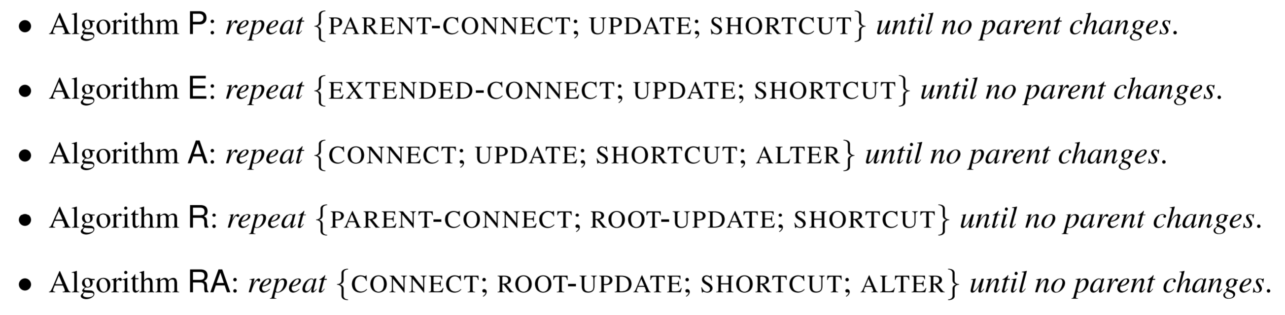
To play with and understand these algorithms, let’s translate the above definitions to Haskell, trying to preserve their clarity and conciseness while also being explicit about details. Jumping ahead a little, here is how Algorithm P will look like in the end:

algorithmP = repeat (parentConnect >>> update >>> shortcut)

Pretty close! Now, let’s define the primitives parentConnect etc. in terms of the underlying computational model where a lot of tiny processing threads communicate via short messages, in rounds. In a round, threads concurrently receive some messages, then update their local states, and possibly send out new messages for the next round. We can capture the local view of a computation round by the following type:

type Local s t i o = s -> t -> [i] -> (s, [(t, o)])

Here s is a type of states, t is a type of threads, and i and o are types of incoming and outgoing messages in a round of computation. In words, given the current state of a thread and a list of incoming messages, a Local function returns an updated state and a list of outgoing messages, each tagged with a target thread identifier — these messages will be delivered in the next computation round.

We can upload Local functions to our tiny processors, say on an FPGA, inject input messages into the communication network, and extract the outputs after a computation round, i.e. when all threads complete the computation. This requires specialised hardware and non-trivial setup, so let’s find a way to simulate such computations on a big sequential machine that has enough memory to have the global view of a round:

type Global s t i o = (Map t s, [(t, i)]) -> (Map t s, [(t, o)])

The Global function takes a map from threads to their current states and a list of all input messages in the network and returns the resulting global state: a map of new thread states and a list of newly generated output messages. Note that such global computations can be composed using function composition and form a category; the operator >>> in the above code snippet for Algorithm P is just the left-to-right composition defined in the standard module Control.Category.

Converting from a Local to a Global view is relatively straightforward:

round :: Ord t => Local s t i o -> Global s t i o
round local (states, messages) = collect (Map.mapWithKey update states)
  where
    deliveries = Map.fromAscList (groupSort messages)
    update t s = local s t (Map.findWithDefault [] t deliveries)
    collect    = runWriter . traverse writer

We first find all the deliveries, i.e. lists of incoming messages that should be delivered to each thread, then execute the local update functions of each thread, sequentially (note that this is OK since threads interact only between rounds), and finally, collect outgoing messages of all threads.

To express Tarjan’s algorithms, we will need the generic repeat function that executes a given Global computation repeatedly until thread states stop changing.

repeat :: (Eq s, Eq t) => Global s t Void Void -> Global s t Void Void
repeat g (states, messages)
    | states == newStates = (states, messages)
    | otherwise           = repeat g (newStates, newMessages)
  where
    (newStates, newMessages) = g (states, messages)

Note that we require that the network is quiescent before and after a given computation, as indicated by the type of incoming and outgoing messages i = o = Void. Of course, the computation may be comprised of multiple rounds, which can exchange messages between each other!

Now let’s use the above definitions to express Algorithms P and R from Tarjan’s paper. We’ll have n + m threads corresponding to vertices and edges, whose states will be very minimalistic: edges will have no state at all, and every vertex will store its current parent i.e. the minimum vertex of the connected component to which the vertex is currently assigned.

type Vertex = Int

data Thread = VertexThread Vertex | EdgeThread Vertex Vertex
data State  = VertexState  Vertex | EdgeState

A vertex that is its own parent is called root; all vertices are initially roots. If this reminds you of the disjoint-set data structure you are on the right track! All algorithms follow the same general idea: we start by assigning each vertex to a separate component and then use edges to inform their neighbouring vertices about other reachable vertices in the component, maintaining the invariant that the root of a component is its smallest vertex. As rounds progress, we grow a parent forest, not dissimilar to the forest produced by the depth-first search for our earlier example graph, but now taking advantage of concurrency.

Let’s also create a convenient type synonym for denoting global views of computation rounds involving s = State and t = Thread:

type (~>) i o = Global State Thread i o

We can now express computation primitives, such as connect, where edges inform their neighbours about each other:

connect :: Void ~> Vertex
connect = round $ \s t _ -> case t of
    VertexThread _ -> (s, [])
    EdgeThread x y -> (s, [(VertexThread (max x y), min x y)])

The type Void ~> Vertex says that the round starts with no messages in the network and ends with messages carrying vertices. Vertex threads are dormant in the round, whereas edge threads generate one message each, sending a smaller vertex to the thread corresponding to the larger vertex so that the latter could update its parent. Note that we express the behaviour locally, and then use the function round defined above to obtain its Global semantics.

This connect round can be followed by the update round, where vertex threads process incoming messages, updating their parents accordingly:

update :: Vertex ~> Void
update = round $ \s _ i -> case s of
    VertexState p -> (VertexState $ minimum (p : i), [])
    EdgeState     -> (s, [])

The primitives connect and update are not sufficient on their own; we need another crucial ingredient — the shortcut primitive that halves the depths of trees in the parent forest, similarly to the path compression technique used in the disjoint-set data structure.

shortcut :: Void ~> Void
shortcut = request >>> respondParent >>> update
  where
    request :: Void ~> Thread
    request = round $ \s t _ -> case s of
        VertexState p -> (s, [(VertexThread p, t)])
        EdgeState     -> (s, [])

respondParent :: Thread ~> Vertex
respondParent = round $ \s _ i -> case s of
    VertexState p -> (s, map (,p) i)
    EdgeState     -> (s, [])

In shortcut, every vertex requests the parent of its parent sending itself as a “respond-to” address. In the subsequent round, each vertex thread responds by sending its parent. The process completes by running the update primitive defined above. Note how we can compose simple primitives together in a type-safe way, obtaining a non-trivial shortcut.

The last primitive that I’ll cover is parentConnect, a variation of connect that informs the parents of two edge vertices about each other:

parentConnect :: Void ~> Vertex
parentConnect = request >>> respondParent >>> receive
  where
    request :: Void ~> Thread
    request = round $ \s t _ -> case t of
        VertexThread _ -> (s, [])
        EdgeThread x y -> (s, [(VertexThread x, t), (VertexThread y, t)])

    receive :: Vertex ~> Vertex
    receive = round $ \s _ i -> case s of
        VertexState _ -> (s, [])
        EdgeState     -> case i of
            [x, y] -> (s, [(VertexThread (max x y), min x y)])
            _      -> error "Unexpected number of responses"

We start by requesting parents of edge vertices, continue by sending the responses using the respondParent primitive defined above, and finally receive and handle the responses in a way similar to connect.

All the ingredients required for expressing Algorithm P are now in place:

algorithmP :: Void ~> Void
algorithmP = repeat (parentConnect >>> update >>> shortcut)

Great! My favourite algorithm from the paper is Algorithm R, which is a slight variation of Algorithm P:

algorithmR :: Void ~> Void
algorithmR = repeat (parentConnect >>> rootUpdate >>> shortcut)

Here we use rootUpdate instead of update, whose only difference is that updates to non-root vertices are ignored. This makes the growth of the parent forest monotonic: we never exchange subtrees between trees and only graft whole trees to other trees. This greatly simplifies the analysis of the performance of Algorithm R compared to Algorithm P. In fact, according to Tarjan, analysis of Algorithm P is still an open problem! I encourage you to read the paper, which presents five (!) algorithms for computing connected components concurrently, and also to implement the two remaining primitives, extendedConnect and alter, required for expressing Algorithms E, A and RA using our little modelling framework.

Let’s check if our implementation of Algorithm P works correctly on the example graph:

initialise :: Graph Int -> Map Thread State
initialise g = Map.fromList (vs ++ es)
  where
    vs = [ (VertexThread x, VertexState x) | x      <- vertexList g ]
    es = [ (EdgeThread x y, EdgeState    ) | (x, y) <- edgeList   g ]

run :: Global s t Void Void -> Map t s -> Map t s
run g m = fst $ g (m, [])

components :: Map Thread State -> [(Int, [Int])]
components m = groupSort
    [ (p, x) | (VertexThread x, VertexState p) <- Map.toList m ]

λ> mapM_ print $ components $ run algorithmP $ initialise example
(1,[1,2,3,4,5,6,7,8,9,10,11,13,15,18,22,23,24,25,27,29,31,32,35,38])
(12,[12,14,16,17])
(19,[19,20,21,26,28,30,33,34,36,37])

As expected, there are three components with roots 1, 12 and 19, which matches the figure at the top of the blog post.

And here is an animation of how Algorithm R builds up the parent forest in a monotonic manner. Note that the edges in the parent forest are now shown as undirected (unlike in the earlier depth-first search figure) since they may change their logical direction during the execution of the algorithm (e.g. see the edge 4-9).

That’s all for now! I hope to find time soon to try these algorithms on Tinsel, a multi-FPGA hardware platform with thousands of processors connected by a fast network. Tinsel is being developed at the University of Cambridge as part of the POETS research project, which I worked on while at Newcastle University. Tinsel is very cool! Have a look at it if you are into FPGAs and unconventional computing architectures.

P.S.: If you haven’t heard about the Heidelberg Laureate Forum before, you can read about it here. If you are a young researcher in computer science or mathematics, you should consider applying — it’s an amazing event where you get a chance to talk to the leaders of the two fields, as well as to young researchers from all over the world. This year I’m here as part of the HLF blogging team, writing about people I met and things I learned here, and it’s been a lot of fun too — if you’d like to help cover and promote this event, get in touch with the HLF media team.

P.P.S.: And here are a couple of links: (i) a video recording of Tarjan’s HLF lecture and (ii) the complete source code from this blog post.