As part of the School of Civil Engineering and Geosciences involvement in University student recruitment activities, prospective 6th form and college students can attend Open and Visit Days. These days give students the opportunity to come and learn a little bit more about the courses that are offered at the University, including those taught within the School. Within Geomatics, prospective students are given some experiences of what it might be like to study Geographic Information Science (GIS), or Surveying and Mapping Science (SMS) Undergraduate courses via a handful of taster exercises. These exercises are designed to enable staff members to talk about some of the basic concepts that a prospective student might learn about should they decide to apply and study GIS or SMS.
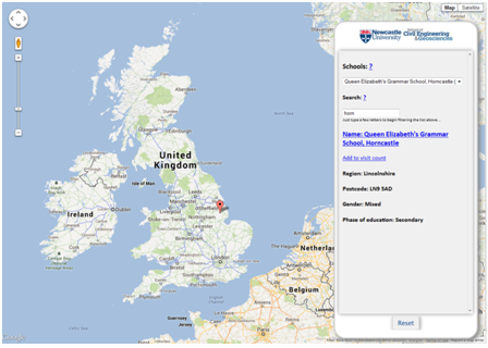
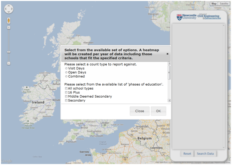
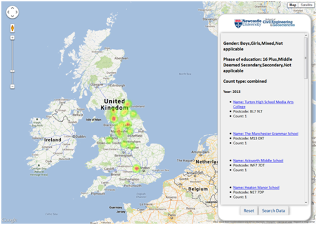
A key student recruitment activity within the School and more widely the University, involves the coordinated marketing and distribution of promotional materials focussed on Undergraduate courses to different colleges and schools around the UK. In order to better understand how the School’s involvement in this activity leads to prospective students attending the University Open and Visit Days, thus showing an interest in the courses on offer from the School, a very simple web-based tool has been developed to record where prospective students are travelling from on Visit and Open Days, by recording against the school or college at which the student attends. However not only does this begin to allow recruitment staff to understand how marketing activities are leading to prospective students attending the Visit and Open Days, it also doubles as a taster exercise in explaining some of the basic concepts of data capture, management and visualisation that a student would learn more about within the GIS and SMS courses. A prospective student is able to search for the school or college that they attend from a geocoded set of more than 60,000 schools, and then subsequently increment a count against that particular school for the particular year in which they attended a Visit or Open Day. All this information is stored within a PostGIS-enabled PostgreSQL relational database, and is served out to the webpage via JSON following the use of standard SQL queries to query the underlying data. As a result a prospective student, as well as recruitment staff, are able to create custom Heat Maps (intensity, not temperature!), all powered by the Google Maps API, of their data, or data from previous years. The query interface allows different HeatMaps to be created based on sub-selections of school type, gender (boys only, girls only, or mixed gender schools) and years of interest.
For clarification the database stores no other information about the student other than a count against a particular school or college at which the prospective student attends, and the addition of new information is protected behind a username and password. The following images give some illustrations of this interface and tool:
Increment count against a school, at which a prospective student attends
During the early summer of 2013, the UK Infrastructure Transitions Research Consortium (ITRC) underwent a mid-term review, approximately two and half years after the inception of the research programme, which coincided with the annual ITRC Assembly. The assembly and review gave all of those working within the consortium, and also invited guests and delegates, the opportunity to hear about the work accomplished during the initial half of the research programme. The 5 year research consortium is funded through an EPSRC Programme Grant, with the mid-term review offering the chance to discuss the future of the flexible funding available for the final two and half years of the programme.
The three day meeting was held at Chilworth Manor Hotel in Southampton, and was facilitated by a facilitation group, Dialogue Matters to help coordinate and focus a delegation of researchers, academics, stakeholders and partners. Monday offered the chance for the Expert Advisory Group (EAG) to review the documentation and work completed under the five different work streams. Whilst part of this review took place behind closed doors alongside the program’s principal and co-investigators, subsequently the EAG gave direct feedback to all of those attending the three day meeting. This session was then followed by an open floor discussion and questioning by researchers, PhD students and investigators from the program of the EAG panel. The utility of the EAG in particular was felt by the program during these discussions, and also via their continued guidance on the cycle 2 and 3 assessments due for release in January 2014 and in the autumn of 2015 respectively. Further to the feedback delivered, the post-lunch slot was dedicated to researchers and investigators funded through the program the chance to present some more specifics about the tasks undertaken during the first half of the program. This was particularly effective in getting everyone up to speed with what others within the consortium had been working on, and helped certainly to set the scene for discussions about future directions assigned to day two and three. Finally, a group of ITRC-affiliated PhD students presented some scoping research they had carried out to try to pull together a set of data on projects, research centres and institutes at the global scale who are also working on similar research as that conducted under the ITRC banner. Not only was the presentation interesting in the manner in which it was delivered, the data and information collected offered a great starting point for further development of the ever-growing research community, acting as a focal point for information about the community at large.
Day two began to offer the affiliated researchers and investigated across the many universities represented within the program, the opportunity to address some of the following questions:
Where have we got to?
What is happening in this field, in other projects and around the world?
What externalities may adjust the way this research is conducted, or will influence the likely impact the research has e.g. changes in policy, education, funding, society, environment, markets etc)
Whilst discussions of these questions began immediately in the morning session to broaden the horizon of future possible directions, a selection of “seed” ideas or possible projects that were a priori selected as being potential key research directions were also considered. The opportunities to think more broadly about possible research directions for the final two and half years of the project and also consideration of ideas already identified as of interest, gave everyone the chance to give their opinion on what could or could not feasibly be achieved given the available remaining time and resource. From a personal perspective, I think this gave everyone a real sense of ownership of the future direction of the research and certainly helped to gauge the relative importance of the different tasks identified by researchers from wholly different backgrounds. Subsequently this session allowed researchers to consider new ideas and areas based on the knowledge gained during the first half of the program. The breadth of ideas was enormous, ranging from the need for autonomous analytics for infrastructure planning, provision, monitoring and recovery to the need for new systems to manage the proposed integration of unmanned aerial vehicles within commercially used airspace in the United States, currently being considered by FAA.
Whilst the majority of the second day was spent considering the future direction of program, the afternoon session gave an opportunity for those involved to take stock of the success of the mechanisms employed for internal communication within the consortium. As the consortium is spread over many research centres and universities, effective communication between them and within the consortium is critical to ensuring objectives are achieved. The qualitative review considered the utility of using social media to facilitate communication both internally and externally, such as the use of Twitter and Skype for external dissemination and internal discussions, whilst also appraising the use of the ITRC intranet for collaborative working, and assessing the state of the external facing ITRC website.
With Tuesday giving plenty of opportunity to widen the research agenda and look at possible future research directions that the consortium could move in to, as well as assessing what tasks are to be achieved within the remaining two and half years of the project, Wednesday’s agenda focussed on narrowing this scope. A series of research themes had been identified from Tuesday’s discussions, and researchers were invited to select a theme upon which to discuss what the key areas of interest within that theme might be. However, not only were ideas generated, but challenges to achieving success in these areas were also highlighted, to give an impression of the relative difficulty of each theme. The results of many of the discussions held on day two and three have certainly helped the principal and co-investigators of the program to coordinate what tasks and objectives are to be achieved within the final years of the program.
Overall the assembly and mid-term Review offered everyone involved in the program to take stock of the achievements to date, whilst recognising the significant challenges that lay ahead when trying to deliver on a program which is trying to understand the complex nature of infrastructure, how it is operated, and it’s likely resilience to impending changes in demography, economy and climate.
The following table offers a summary of those people who were involved in the three day meeting:
As the ITRC programme progresses and approaches the mid-term review stage, in June and July of 2013, the of the work stream 1 (WS1) infrastructure capacity and demand modelling teams are beginning to produce outputs from their next round of modelling. Furthermore, the parallel development of spatial infrastructure networks as part of work stream 2 (WS2), is beginning to raise some significant challenges in terms of appropriate and effective data dissemination, communication and interpretation. The underlying high-dimensionality nature of the data being produced as part of WS1 for example, coupled with the complexity of the networks generated as part of WS2 means the consortium as a whole needs to begin to think about appropriate mechanisms to visualise these data. For example, some initial prototypes of possible visualisation tools are beginning to be developed, (see here), but rather than build and design tools from the perspective of one researcher, it was considered more appropriate to consult with, other similar projects who are visualising similar data, or will require the ability to visualise similar data in similar ways to that required of ITRC, and also a host of visualisation and design experts from around the UK to gain better perspectives.
An initial workshop, organised by ITRC members, Dr Alex Otto (ITRC WS1 investigator), Dr Greg McInerny (Senior Research Fellow, University of Oxford), Mr David Alderson (Researcher in GeoInformatics, Newcastle University), Dr Stuart Barr (Senior Lecturer in Geographic Information Science, Newcastle University) and Miriam Mendes (ITRC Programme Manager, University of Oxford), sought to bring together relevant researchers from the plethora of Adaptation and Resilience in a Changing Climate (ARCC) network projects and leading researchers and experts in the field of data visualisation and design. Prior to the workshop, a questionnaire was distributed to both the invited ARCC project representatives and the visualisation experts in an attempt to give the organising team a better centralised perspective of what the respective groups would want to hope to gain by attending the workshop. The responses were then studied to teaseout any overlaps between visualisation challenges faced across the ARCC projects, to attempt to collate a set of discussion points upon which to focus discussions in the afternoon of the workshop. Prior to these more focussed discussion sessions, the workshop initially allowed the ARCC project representatives to briefly (in 5 minutes or less) explain the nature of the project in which they are working, but also describe and explain some of the visualisation challenges being faced within that project. The aim of this early session was to allow the visualisation experts time to understand the background of the projects themselves, and also the nature of some of the data being produced, such that the more focussed discussions taking place in the afternoon had a little context.
From the responses to the questionnaire, and also following the morning’s ARCC project overview session, a series of 5 discussion topics were devised, that attempted to encapsulate the common visualisation challenges across all the projects, and are listed below.
Temporal visualisation of infrastructure behaviour and response;
Chair: Sean Wilkinson (RESNET – Newcastle University)
Rapporteur: Min Chen (Visualisation – University of Oxford)
Simplifying and communicating effectively complex model outputs;
Chair: Jason Dykes (Visualisation – City University, London)
Rapporteur: Scott Kelly (ITRC – Cambridge University)
Multi-disciplinary co-production for infrastructure visualisation.
Chair: Simon Blainey (ITRC – University of Southampton)
Rapporteur: Jane Lewis (Reading e-Science Centre, University of Reading)
A chair and rapporteur, selected from the list of workshop attendees was devised such that each topic had a representative from the ARCC network, and from the visualisation community. Each topic was then discussed by attendees for about 10 minutes, with the chairs and rapporteurs capturing the salient points discussed around that particular topic. After 10 minutes of discussion the attendees subsequently moved on to the next discussion topic and a different table. Overall as a format for delivering break out sessions, this quick-fire, round-robin approach seemed to work well, allowing all attendees to discuss all the common discussion topics about visualisation, whilst at the same time having the discussions steered and reported by representation from both sides. The approach also seemed to help stimulate discussions between project representatives and visualisation experts, which was one of the objectives or organising and delivering the workshop. However further work is currently being undertaken to transform some of the excellent discussions in to a positioning paper with respect to visualising high dimensionality data for infrastructure planning and provision purposes. It is hoped that representatives from the projects, particularly those organising the workshop and on the ITRC side will be looking to further engage and collaborate with the visualisation community. Watch this space…
Links to presentations split by those relevant to different communities are listed below:
ARCC Projects presentations and speakers listed below
As many of the networks that I am building as part of my involvement in the Infrastructure Transitions Research Consortium (ITRC – www.itrc.org.uk) are inherently spatial, I began thinking about how it might be useful to be able to visualise a network using the underlying geography but also as an alternative, the underlying topology. I began exploring various tools, and libraries and just started playing around with D3 (d3js.org). D3 is a javascript library that offers a wealth of widgets and out-of-the-box visualisations for all sorts of purposes. The gallery for D3 can be found here. As part of these out-of-the-box visualisations it is possible to create force directed layouts for network visualisation. At this stage I began to think about I can get my network data, created by using some custom Python modules, nx_pg and nx_pgnet and subsequently stored within a custom database schema within PostGIS (see previous post here for more details), in a format that D3 can cope with. The easiest solution was to export a network to JSON format as the nx_pgnet Python modules allow a user to export a networkx network to JSON format (NOTE: the following tables labelled “ratp_integrated_rail_stations” and “ratp_integrated_rail_routes_split” were created as ESRI Shapefiles and then read in to PostGIS using the “PostGIS Shapefile and DBF Loader”).
Having exported the network to JSON format (original data sourced from http://data.ratp.fr/fr/les-donnees.html), this was then used as a basic example to begin to develop an interface using D3 to visualise the topological aspects, and OpenLayers to visualise the spatial aspects of the network. A simple starting point was to create a basic javascript file that contained lists of networks that can be selected within the interface and subsequently viewed. Not only did this include a link to the underlying file that contained the network data, but also references to styles that can be applied to the topological or geographic views of the networks. A series of separate styles using the underlying style regimes of D3 and OpenLayers were developed such that a style selectable in the topological view used exactly the same values for colours, stroke widths, fill colours as styles applicable in the geographic view. These stylesheets, stored within separate javascript files are pulled in via an AJAX call using jQuery to the webpage, subsequently allowing a user to select them. Any numeric attributes or values attached at the node or edge level of each network could also subsequently be used as parameters to visualise the nodes or edges in the networks in either view e.g. change edge thickness, or node size, for example. Furthermore, any attribute at the node or edge level could be used for label values, and these various options are presented via a set of simple drop down menu controls on the right hand side of the screen. As you may expect, when a user is interested in the topological view, then only the topological style and label controls are displayed, and vice versa for the geographic view.
For spatial networks, the geographic aspects of the data are read from a “WKT” attribute attached to each node and edge, via a WKT format reader to create vector features within an OpenLayers Vector Layer. It is likely this will be extended such that networks can be loaded directly from those being served via WMS, such as through Geoserver, rather than loading many vector features on the client. However for the purposes of exploring this idea, all nodes and edges within the interface on the geographic view can be considered as vector features. The NodeID, Node_F_ID, and Node_T_ID values attached to each node, or edge respectively as a result of storing the data within the custom database schema, are used to define the network data within D3.
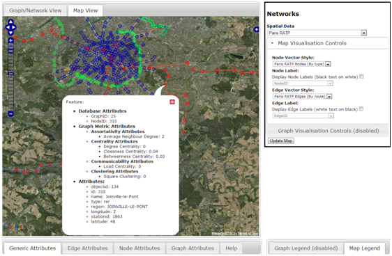
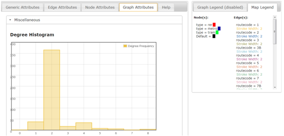
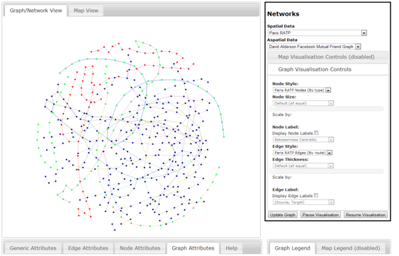
At this stage it is possible to view the topological or geographic aspects of the network within a single browser pane. Furthermore, if graph metrics have been calculated against a particular network and are attached at either the whole graph, or individual node or edge level, they too can be viewed within the interface via a series of tabs found towards the bottom. The following image represents an example of visualising the afore-mentioned Paris Rail network using the interface, where we can see that the controls mentioned, and how the same styles for the topological and geographic views are making it easier to understand where one node or edge resides within the two views. The next stage is to develop fully-linked views of a network such that selections made in one window are maintained within another. This type of tool can be particularly useful for finding disconnected edges via the topological view, and then finding out where that disconnected edge may exist in it’s true spatial location.
Example of the geographic view of the Paris Rail Network displayed using OpenLayers (data read in from JSON objects, with geometry as WKT)
Example of graph metrics (degree histogram) for Paris Rail Network (data stored at network level)
Example of the topological view of the Paris Rail Network displayed using force directed layouts from D3.js
The location of the football team that you support is often a cause for debate, with chants like “we support our local team” being heard on the terrace week in week out. And now with the influx of football fans taking to twitter to support their teams this provides another way of measuring this metric.
As a group the idea of using twitter to crowd source the location of events is not a new one. Previously we have used it to record flood events across the north east allowing for a real time map to be produced. An idea which will be used heavily in the forthcoming iTURF project (integrating Twitter with Realtime Flood modelling).
So for me to develop a football script it was simply a matter of applying our previously developed scripts to record the locations of tweets related to football teams. For this I used the official hashtag for each team and then simply recorded the club, location and time, the actual body of the tweet is not stored.
Once this script was in place and I had the data feeding into a database I was able to develop a webpage displaying the tweets in real-time.
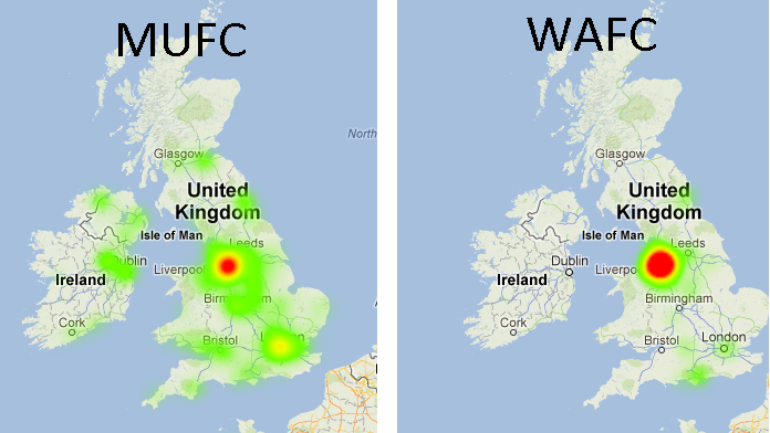
As well as this by using the google maps api I was also able to produce heat maps for each club. Showing the hotspots for the support of each team, predictably some show more spread than others.
Analysing a section of tweets also revealed some interesting statistics the club with the lowest average distance from tweet (uk based only) to their home ground was Fulham and Newcastle who pride themselves in their local support were the second furthest away.
club
Average distance in km
Fulham FC
81.64537729
West Ham United FC
82.46339901
West Brom Fc
82.78354779
Wigan Athletic
109.7845034
Tottenham Hotspur
112.3828775
Southampton FC
121.436554
Stoke City
123.7468635
Manchester City
128.4830384
Chelsea
134.4779064
Reading Football Club
141.2626039
Arsenal FC
147.5236349
Aston Villa Football Club
148.2891941
QPR
157.5900255
Swansea
162.7745008
Norwich City
164.774284
Sunderland
172.5479224
Everton
176.5113378
Manchester United
184.157026
Newcastle United
203.0311727
Liverpool
209.1425266
However analysing the proportion of tweets by county about team in their county, it revealed that almost 85% of the recorded football tweets in the Tyne and Wear region were about either Sunderland or Newcastle. Whilst Norfolk, which is said to be a one team county, had only 47% of the recorded tweet mentioning Norwich City.
County
Teams
Proportion about teams
Tyne and Wear
Sunderland & Newcastle
84.54%
Haringey
Tottenham Hotspur
74.83%
Manchester
Machester United & Manchester City
64.44%
Merseyside
Liverpool & Everton
63.86%
Hammersmith and Fulham
QPR & Chelsea
62.79%
Southampton
Southampton
61.80%
Stoke-on-Trent
Stoke
48.25%
Norfolk
Norwich
46.99%
West Midlands
West Brom & Aston Villa
36.12%
Islington
Arsenal
30.00%
Newham
West Ham
18.52%
Berkshire
Reading
18.35%
Swansea**
Swansea
11.11%
Richmond upon Thames
Fulham
8.51%
**Note the low proportion for Swansea is suspected to be due to the clash with Stoke City. Whilst Stoke City hashtag is #scfc and Swansea City’s is #swansfc are large number of #scfc are still recorded in south wales.
The hope is for this work whilst relatively simple and rather unscientific it demonstrates what can be achieved by using twitter as a source of information. It also provides a good way of load testing our code and backend database that we will use in the iTURF project
In order to establish a long term urban research facility Newcastle University is looking to bring together new and existing data that includes the urban climate, air quality, pedestrian and traffic flows as well as hydraulic flows. These new data sources will come from a number of sources, one of which will be a system of new sensors set-up around Newcastle. The particular sensors that are going to be used are waspmotes developed by Libelium, sensor devices specially oriented to developers. They work with different protocols (ZigBee, Bluetooth and GPRS) as well as a variety of frequencies (2.4GHz, 868MHz and 900MHz). More than 50 sensors can be connected with these devices with the measurements and frequency configured manually. The sensors can take a number of readings such as the concentration of different gases, temperature, liquid level, weight, pressure, humidity, luminosity, accelerometer, soil moisture and solar radiation.
Thus, as part of my role as a research assistant on this project I was sent along to a training course learning how to write the code to configure these devices. The training course took place in Zaragoza, Spain at Libelium HQ.
It consisted of 4 days of demonstrations and exercises getting familiar with the equipment and how to use them. These ranged from getting the waspmote to send “hello world” to a gateway (a USB device that receives messages and prints them to the screen) all the way through to sensing nearby Bluetooth devices then sending these to a database. We were also taught “clever” uses of the sensors like using the internal accelerometer to detect whether the device had fallen or was being stolen (attach a GPS and a SIM card and you can get it to text you the thief’s location!).
At the end of the training course we were shown their next generation of sensors; the Plug and Sense. These require very little development work as the devices come already mounted in a box and the user just has to attach the relevant sensor probe and then use the code generator to set the recordings taken and frequency at which they are taken.
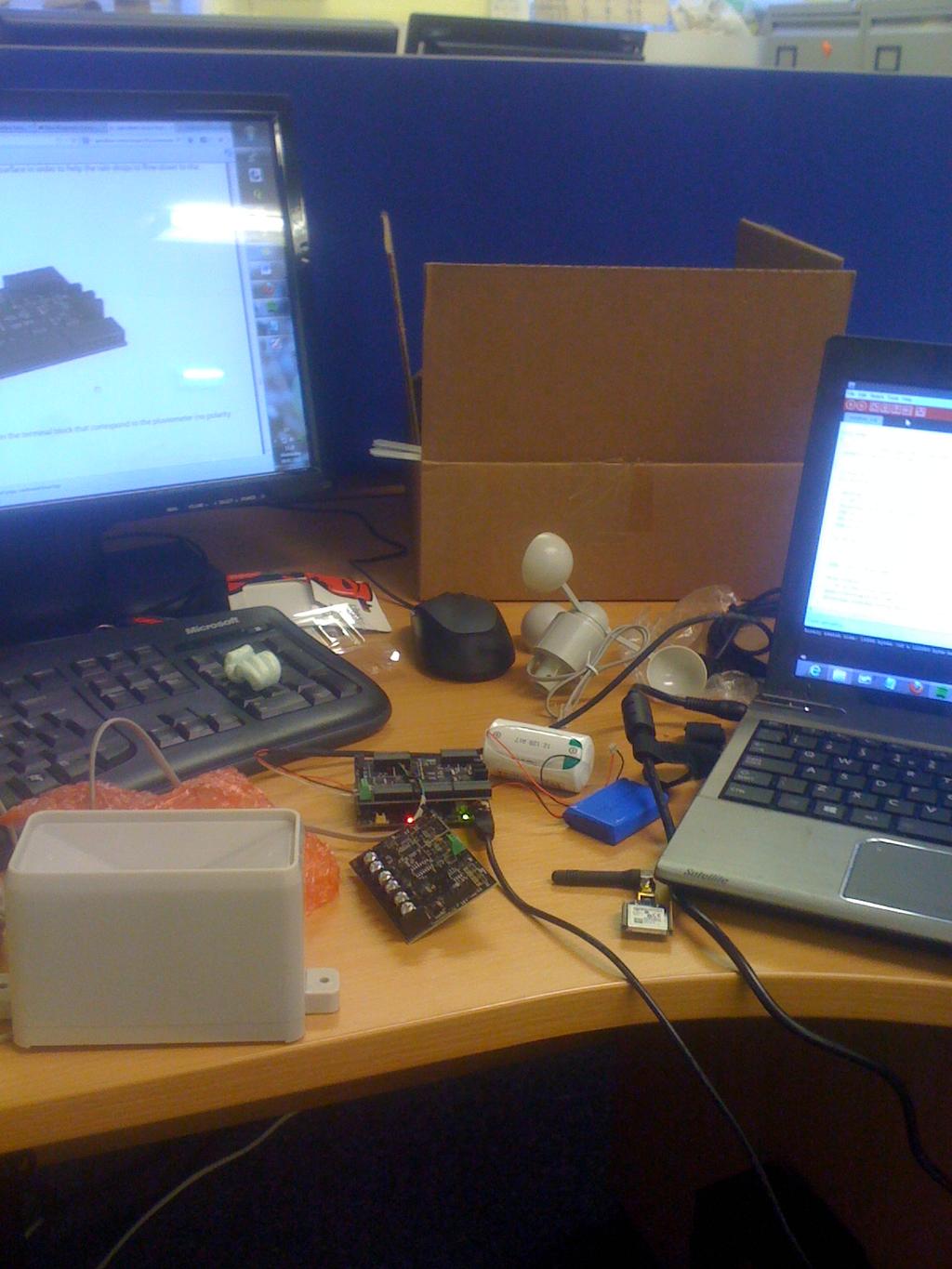
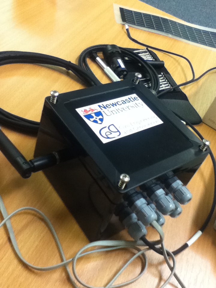
Since returning I have started to develop a weather station using a waspmote, an agriculture board and weather sensors such as a rain gauge, an anemometer and a temperature gauge.
My cluttered desk whilst developing the weather station
Despite initial setbacks, like recording monsoon like conditions whilst inside, I was able to get it set up and feeding into a postgres database. From this, I set-up a simple webmap using the database along with django to display the location of the sensor and the data feed.
The first version of web map and data feed
The aim is now to develop more sensors and deploy these in more meaningful places (not everybody just wants to know the temperature in my office) around the University campus and wider city.
Weather proof box for the deployment of the sensors
The recent upgrade to PostGIS has caused some issues with geometry types when creating views from geometry that don’t use the new typemod geometry modifiers. The following workaround correctly inserts an entry into the geometry_columns view so you can see your data in QGIS and the like:
DROP VIEW myview;
CREATE OR REPLACE VIEW myview AS (
SELECT field1, field2, field3,
St_Transform(the_geom, 27700)::geometry(Point, 27700) as the_geom
Identifying the pattern trends of temperature in a city of a difficult and challenging subject, though through the use of Advanced Very High Resolution Radiometer (AVHRR), our researchers have shown the extent of the variability across a major city can be tremendous. Using data for London, it has been shown that there is a high degree of sensitivity to local meteorological effects and daily cycles.
Comparison of the Urban Heat Island Intensity (UHII) [the maximum difference between urban and rural temperatures during one day] in a statistically robust manner showed that the 2003 heatwave UHII data sets for both image surface and ground air temperatures did not exhibit significantly greater intensities than the other years under consideration. This is in contrast to other work on this topic (e.g. Cheval et al., 2009; Tomlinson et al., 2010) that indicates that not only is the UHII metric a relatively poor means by which to distinguish between a heatwave summer in London, but also the need for further scrutiny of the use of the UHII.
Two members of the Geospatial Engineering team (David Alderson and Craig Robson) were due to present their current infrastructure/network-related research at the recent ITRC Early Career Researcher’s conference, held at Cambridge University on November 27th 2012. As such both embarked on a journey, departing from Newcastle at 0556 on the morning of the 27th, that would end having only reached as far South as Darlington…approximately 6 hours after departing! The cause of being only able to travel a few miles in that time…a flood-related failure of the rail network leading to a loss of power to the train and line between Durham and Darlington. A set of images taken on the day of the failure illustrate the researcher’s plight.
On the 26th October, as part of the monthly Geospatial Engineering meeting, I presented an update on some of my research thus far, since beginning my PhD last September. The presentation focused on some of the more recent research I have been doing, associated with identifying a hierarchical structure in networks. Below is a summary of the work and a note on future presentations.
It is acknowledged in infrastructure literature that some infrastructures have a hierarchical structure, different from the traditional theoretic network structures. These include common models like the random model, scale-free and small-world structures. The main difference between graph structures is the distribution of node degree, the proportion of nodes which are connected to a certain number of edges. A hierarchical structure (looks like a tree) would be expected to have some sort extra organization in it, leading to an underlying hierarchical structure, such as a tree. If it can be shown that this is true and hierarchical networks can be identified, it may be shown that the structure of these are significant and thus may allow for the improvement of the resilience of such networks.
The research utilised the networkx python library, a complex network package. This allowed for the creation of the common network structures mentioned earlier, as well as for the analysis of these through an extensive collection of analysis algorithms. To create a better representation of hierarchical networks, two in-house algorithms were developed to soften he transition between random networks and the balanced tree network, an explicit hierarchical network.
The first set of analysis was performed using common graph metrics such as degree (the number of edges connected to a node) and the average shortest path across a network. A suite of graphs were created for this analysis which covered a range of sizes and complexities for all graph types. This led to the identification of a pair of metrics, which in combination, allowed hierarchical networks to be separated from the other graph structures in the analysis. (The metrics which were identified are the assortativity coefficient and the max betweenness centrality value).
The accuracy of this was confirmed through a series of statistical test, for all pair wise combinations, including chi-squared tests as well as transformed divergence tests to compare the distribution patterns of the metrics of all graph types. In the majority of cases it was shown that the distributions for the graph types did not match in many cases, and there was a significant difference between the rest and the hierarchical structures.
This shows that there is a significant difference between the structure types and thus further investigation into the significance of this, as planned, is worth while completing as there could be future implications on the resilience and design of infrastructure networks. This work will involve resilience analysis of the range of network structures so the results can be compared and the significance quantified. In the longer term this work will be applied onto real-world networks.
A similar presentation with recently completed work will be presented at the ITRC Early Career Researchers Conference at the end of November.